Story

How to filter in excel by columns. Advanced filter in Excel and examples of its features

Probably all users who constantly work with Microsoft Excel are aware of such useful function this program as data filtering. But not everyone is aware that there are also advanced features of this tool. Let's take a look at what Microsoft Excel advanced filter can do and how to use it.

It is not enough to immediately run the advanced filter - for this, one more condition must be met. Next, we will describe the sequence of actions that should be taken.

Step 1: Create a table with selection criteria

To install an advanced filter, first of all, you need to create an additional table with selection conditions. Her hat is exactly the same as the main one, which we, in fact, will filter. For example, we placed an additional table above the main one and colored its cells orange. Although you can place it in any free space and even on another sheet.

Now we enter in the additional table the information that will need to be filtered from the main table. In our particular case, from the list of wages issued to employees, we decided to select data on the main male staff for 07/25/2016.

Step 2: Running the advanced filter

Only after the additional table has been created, you can proceed to the launch of the advanced filter.

Thus, we can conclude that the advanced filter provides more options than regular data filtering. But it should be noted that working with this tool is still less convenient than with a standard filter.

The main drawback of the standard ( ) is the absence of visual information about the applied this moment filter: every time you need to go into the filter menu to remember the criteria for selecting records. This is especially inconvenient when multiple criteria are applied. The advanced filter does not have this drawback - all criteria are placed in a separate table above the filtered records.

Creation algorithm advanced filter simple:

Create a table to which the filter will be applied (source table);
We create a plate with criteria (with selection conditions);
We launch Advanced filter.

Let in the range A 7:S 83 there is an initial table with a list of goods containing fields (columns) Product, Quantity and Price(see example file). The table must not contain empty rows and columns, otherwise Advanced filter(and normal ) will not work correctly.

Task 1 (starting...)

Set up a filter to select rows that contain values in the name of the Product beginning from the word Nails. This selection condition is satisfied by lines with goods nails 20 mm, Nails 10 mm, Nails 10 mm and Nails.

BUT 1 :A2 A2 indicate the word Nails.

Note: Criteria structure y advanced filter is clearly defined and it coincides with the structure of criteria for the functions BDSUMM() , COUNT() , etc.

Usually the criteria advanced filter are placed above the table to which the filter is applied, but they can also be placed on the side of the table. Avoid placing a label with criteria under the original table, although this is not prohibited, it is not always convenient, because new rows can be added to the original table.

ATTENTION!
Make sure that there is at least one empty line between the table with the values of the selection conditions and the original table (this will make it easier to work with advanced filter).

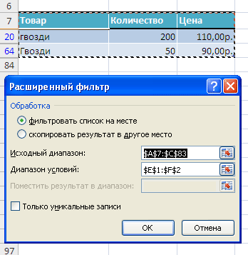
Advanced filter:

call Advanced filter();
in field original range A 7:S 83 );
in field Range of conditions BUT1 :A2 .

If desired, you can copy the selected rows to another table by setting the switch to the position Copy the result to another location. But we won't do that here.

Press the OK button and the filter will be applied - only the rows containing the Product name in the column will remain in the table nails 20 mm, Nails 10 mm, Nails 50 mm and Nails. The rest of the lines will be hidden.

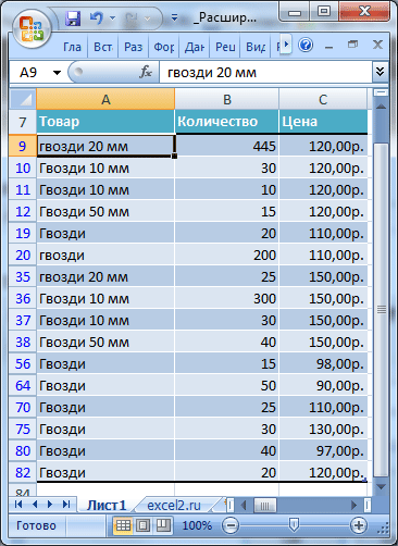
Selected line numbers will be highlighted in blue.

To cancel the filter action, select any cell in the table and click CTRL+SHIFT+L(the title will be applied and the action advanced filter will be canceled) or press the menu button Clear ().

Task 2 (exact match)

Let's set up a filter to select rows that have in the Product column exactly contains the word Nails. This selection condition is satisfied by rows with goods only nails and Nails(does not count). Values nails 20 mm, Nails 10 mm, Nails 50 mm will not be taken into account.

We will place the plate with the selection condition We will place it in the range B1:B2 . The plate should also contain the name of the column heading by which the selection will be made. As a criterion in a cell B2 specify the formula ="= Nails".

Now everything is ready to work with Advanced filter:

select any cell of the table (this is not necessary, but it will speed up filling in the filter parameters);
call advanced filter ( Data/ Sort & Filter/ Advanced);
in field original range make sure the table cell range is specified along with the headers ( A 7:S 83 );
in field Range of conditions specify the cells containing the label with the criterion, i.e. range B1:B2 .
Click OK

Apply Advanced filter with such simple criteria, it makes little sense, because handle these tasks with ease. Autofilter. Let's consider more complex filtering tasks.

If you specify not ="=Nails" as a criterion, but simply Nails, then all records containing names will be displayed beginning from the word Nails ( Nails 80mm, Nails2). To display product lines, containing on word nails, For example, New nails, you need to specify ="=*Nails" as a criterion, or just * Nails where* is and means any sequence of characters.

Task 3 (OR condition for one column)

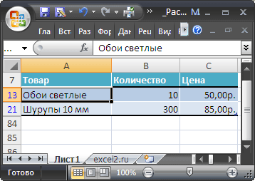
Set up a filter to select rows whose Product column contains a value starting with the word NailsOR Wallpaper.

The selection criteria in this case should be placed under the appropriate column heading ( Product) and should be located one below the other in one column (see the figure below). Place the criteria plate in the range C1:C3 .

The window with the Advanced filter options and the table with the filtered data will look like this.

After clicking OK, all records containing in the column will be displayed Product products Nails OR Wallpaper.

Task 4 (condition AND)

exactly contain in a column Product products Nails, and in the column Quantity value >40. The selection criteria in this case should be placed under the appropriate headings (Product and Quantity) and should be on the same line. Selection conditions should be written in a special format: ="= Nails" and =">40" . We will place the plate with the selection condition We will place it in the range E1:F2 .

After pressing the OK button, all records containing in the column will be displayed Product products Nails with count >40.

ADVICE: When changing the selection criteria, it is better to create a plate with the criteria each time and after calling the filter, only change the link to them.

Note: If you had to clear Advanced Filter options ( Data/ Sort & Filter/ Clear), then before calling the filter, select any cell in the table - EXCEL will automatically insert a link to the range occupied by the table (if there are empty rows in the table, a link will not be inserted to the entire table, but only to the first empty row).

Task 5 (OR condition for different columns)

The previous problems could, if desired, be solved by ordinary . The same problem cannot be solved by a conventional filter.

Let's select only those rows of the table that exactly contain in a column Product products Nails, OR which are in the column Quantity contain a value >40. The selection criteria in this case should be placed under the appropriate headings (Item and Quantity) and should be placed on the different lines . Selection conditions must be written in a special format: ="> 40" and ="= Nails". We will place the plate with the selection condition We will place it in the range E4:F6 .

After pressing the OK button, records containing in the column will be displayed Product products Nails OR value >40 (for any product).

Task 6 (Selection conditions created as a result of applying the formula)

real power advanced filter manifests itself when formulas are used as selection conditions.

There are two options for specifying string selection conditions:

directly enter values for the criterion (see tasks above);
generate a criterion based on the results of formula execution.

Consider the criteria given by the formula. The formula specified as the selection criteria must return TRUE or FALSE.

For example, let's display rows containing a Product that occurs only 1 time in the table. To do this, enter in the cell H2 formula =COUNTIF(Sheet1!$A$8:$A$83,A8)=1, and in H1 instead of heading enter some explanatory text, for example, Non-Duplicate Values. Applicable Advanced filter, specifying the range of cell conditions H1:H2 .

Note that the value search range is entered using , and the criterion in the COUNTIF() function is entered with a relative reference. This is necessary because when using advanced filter EXCEL will see that A8 is a relative reference and will move down the Product column one record at a time and return either TRUE or FALSE. If TRUE is returned, then the corresponding table row will be displayed. If FALSE is returned, the row will not be displayed after applying the filter.

Examples of other formulas from the example file:

Output rows with prices greater than the 3rd highest price in the table. =C8>LARGE($C$8:$C$83 ;5) This example clearly shows the trickiness of the BIGGEST() function. If you sort a column With (prices), we get: 750; 700; 700 ; 700; 620, 620, 160, ... In human terms, "3rd highest price" corresponds to 620, and in the understanding of the GREAT() function - 700 . As a result, not 4 lines will be displayed, but only one (750);
String output case sensitive =EXACT("nails", A8). Only those rows in which the product will be displayed will be displayed. nails entered using lowercase letters;
Output of rows with price higher than average =C8>AVERAGE($C$8:$C$83);

ATTENTION!
Application advanced filter cancels the filter applied to the table ( Data/ Sort & Filter/ Filter).

Task 7 (Selection conditions contain formulas and usual criteria)

Consider now another table from sample file on sheet Task 7.

In column Product the name of the product is given, and in the column Product type- his type.

The task is to display products with a price below the average for a given type of product. That is, we have 3 criteria: the first criterion sets the Product, the 2nd - its Type, and the 3rd criterion (in the form of a formula) sets the price below the average.

We will place the criteria in lines 6 and 7. Enter the required Product and Product Type. For a given Product Type, we calculate the average and display it for clarity in a separate cell F7. In principle, the formula can be entered directly into the criterion formula in cell C7.

2 out of 4 products (of the specified product type) will be displayed.

Problem 7.1. (Are 2 values on the same line the same?)

There is a table that shows the year of manufacture and the year of purchase of the car.

You want to display only those rows in which the Year of issue is the same as the Year of purchase. This can be done using the elementary formula =B10=C10.

Problem 8 (Is a symbol a number?)

Suppose we have a table with a list various types nails.

It is required to filter only those rows whose Product column contains Nails 1 inch, Nails 2 inches etc. products Stainless nails, Chrome-plated nails etc. should not be filtered.

The easiest way to do this is to set a condition as a filter that after the word Nails there should be a number. This can be done using the formula =ISNUMBER(--MID(A11,LSTR($A$8)+2,1))

The formula removes 1 character from the product name after the word Nails (including spaces). If this character is a number (digit), then the formula returns TRUE and the string is displayed, in otherwise line is not output. Column F shows how the formula works, i.e. it can be tested before launch advanced filter.

Task 9 (Output rows that DO NOT CONTAIN the given Goods)

It is required to filter only those rows that do NOT contain in the Product column: Nails, Board, Glue, Wallpaper.

For this you will have to use a simple formula =END(VLOOKUP(A15,$A$8:$A$11,1,0))

Use the AutoFilter or built-in comparison operators such as "greater than" and "top 10" in Excel to show the data you want and hide the rest. After filtering data in a range of cells or a table, you can either reapply the filter to get up-to-date results, or you can clear the filter to re-display all the data.

Use filters to temporarily hide some data in a table and only see the data you want.

Filtering a Data Range

Filtering data in a table

The filtered data only shows rows that match the specified condition and hides rows that you don't want to display. After filtering the data, you can copy, find, modify, format, chart, and print a subset of the filtered data without moving or modifying it.

You can also filter on multiple columns. The filters are additive, which means that each additional filter builds on the current filter and further reduces a subset of the data.

Note: When using the dialog box Search to search for filtered data, only the data that appears in the list is searched. Data that is not displayed is not searched. To find all data, clear all filters.

additional information about filtering

Two types of filters

With autofilter, you can create two types of filters: by list value or by criteria. Each of these filter types is mutually exclusive for each cell range or column table. For example, you can filter on a list of numbers or a condition, but not both; You can filter by icon or custom filter, but not both.

Reapplying a filter

To determine if a filter has been applied, look at the icon in the column heading.

Reapplying a filter produces different results for the following reasons.

Data has been added, changed, or deleted in a range of cells or a table column.

the values returned by the formula have changed and the worksheet has been recalculated.

Don't use mixed data types

For achievement best results You should not mix data types such as text and number, or numbers and dates in the same column, because only one type of filter command is available for each column. If a mixture of data types is used, the displayed command is the data type that is most often invoked. For example, if a column contains three values stored as a number and four stored as text, the command is displayed text filters .

Filtering data in a table

As you enter data into a table, filtering controls are automatically added to its column headers.

Filtering a Data Range

If you don't want to format your data as a table, you can also apply filters to a range of data.

Select the data you want to filter. For best results, columns should contain headings.

On the tab " data"press button" Filter".

Filtering Options for Tables and Ranges

You can apply a general filter by selecting Filter, or a custom filter based on the data type. For example, when filtering numbers, the item is displayed Numeric filters, the item is displayed for dates Date filters, and for text - Text filters. By applying a general filter, you can choose to display the desired data from the list of existing ones, as shown in the figure:

Selecting an option Numeric filters you can apply one of the following custom filters.

Excel data filtering helps you quickly set conditions for the rows that you want to display, and hide the rest of the rows that do not match the conditions.

The filter is set on the headings and subheadings of tables; the main thing is that the cells on which the filter will be installed are not empty. And it is located in the Excel workbook menu on the Data tab, the Sort and Filter section:

By clicking on the "Filter" icon, the upper cells of the range will be defined as headers and will not participate in filtering. Headings will be marked with . Click on it to see the filter options:

Filters in Excel allow sorting. Remember that if you have not selected all the columns of the table, but only some part, and apply sorting, then the data will be lost.

"Filter by color" allows you to select rows in a column that have a specific font or fill color. You can only choose one color.

"Text filters" make it possible to set certain conditions for strings, such as: "equal", "not equal" and others. By selecting any of these items, a window will appear:

You can set the following conditions in it:

The conditions “equal to” and “not equal to” do not require explanation, because everything is very clear with them;
greater than, less than, greater than or equal to, and less than or equal to. How can strings be compared to each other? To understand this, remember how Excel sorts. Those. the further the string is in the sort list, the larger its value. The following statements are true (correct): A<Б; АА>BUT; BUT<=Я; 5 яблок < апельсин.
"starts with", "does not start with", "ends with", "does not end with", "contains", and "does not contain". In principle, the conditions speak for themselves and can take a character or a set of characters as values. Pay attention to the hint in the window located below all the conditions (explanations will follow).

If necessary, you can set 2 conditions using the logical "AND" or "OR".

If "AND" is selected, all conditions must be met. Watch out for conditions that don't exclude a friend, such as "<Значение И >Meaning”, because nothing at the same moment can be both more and less than the same indicator.

When using "OR", at least one of the specified conditions must be met.

A hint is provided at the very end of the Custom AutoFilter window. Its first part: "The question mark ""?"" denotes any one character ... ". Those. when setting conditions when it is impossible to accurately determine the character in a particular place in the string, substitute "?" in its place. Condition examples:

Starts with "?va" (starts with any character followed by "va") will return the results: "Ivanov", "Ivanova", "quartz", "svat" and other strings that match the condition;
Equals "???????" - will return as a result a string that contains 7 any characters.

The second part of the hint: "The sign ""*"" denotes a sequence of any characters." If it is impossible to determine in the condition which characters and in what quantity should be in the string, then substitute "*" instead. Condition examples:

Ends with "o * t" (ends with "o" followed by any sequence of characters, then the character "t") will return the result: "sweat", "cake", "turnover" and even this - "rvnschuoooviunistvrunkt".
Equal to "*" - will return a string that contains at least one character.

In addition to text filters, there are “Number filters”, which basically accept the same conditions as text filters, but also have additional ones related only to numbers:

Above Average and Below Average - Returns values that are above and below the average, respectively. The average value is calculated from all the numeric values in the column list;
“First 10…” – clicking on this item brings up the window:

Here you can specify which elements to display the first of the largest or the first of the smallest. Also, how many items to display if the item "list items" is selected in the last field. If the item "% of the number of elements" is selected, the second value specifies this percentage. Those. if there are 10 values in the list, then the highest (or lowest) value will be selected. If there are 1000 values in the list, then either the first or last 100.

Microsoft Excel is a ubiquitous and user-friendly spreadsheet tool. Wide functionality makes this program the second most popular after MS Word among all office programs. It is used by economists, accountants, scientists, students and representatives of other professions who need to process mathematical data.

One of the most convenient features in this program is data filtering. Consider how to set up and use MS excel filters.

Where are filters in Excel - their types

Finding filters in this program is easy - you need to open the main menu or just hold down the Ctrl + Shift + L keys.

How to set a filter in Excel

Basic filtering functions in Excel:

filter by color: allows you to sort data by font or fill color,
text filters in excel: allow you to set certain conditions for rows, for example: less than, greater than, equal to, not equal to, and others, as well as set logical conditions - and, or,
numeric filters: sort by numeric conditions, such as below average, top 10, and others,
manual: selection can be made according to self-selected criteria.

They are easy to use. It is necessary to select the table and select the section with filters in the menu, and then clarify by what criterion the data will be screened.

How to use advanced filter in Excel - how to customize it

The standard filter has a significant drawback - in order to remember which selection criteria were used, you need to open the menu. And even more so it causes inconvenience when more than one criterion is set. From this point of view, an advanced filter is more convenient, which is displayed as a separate table above the data.

VIDEO INSTRUCTION

Setting order:

Create a table with data for further work with it. It should not contain empty lines.
Create a table with selection conditions.
Run advanced filter.

Let's look at an example setup.
We have a table with columns Product, Quantity and Price.

For example, you need to sort rows whose product names begin with the word "Nails". Several rows fall under this condition.

The table with the conditions will be placed in cells A1:A2. It is important to indicate the name of the column where the selection will take place (cell A1) and the word itself for selection - Nails (cell A2).

It is most convenient to place it above the data or on the side. It is also not forbidden under it, but it is not always convenient, since from time to time it may be necessary to add additional lines. Indent at least one blank line between the two tables.

Then you need:

select any of the cells
open the "Advanced filter" along the path: Data - Sort and filter - Advanced,
check what is specified in the "Initial range" field - the entire table with information should go there,
in the "Range of conditions" it is necessary to set the values of the cells with the selection condition, in this example it is the range A1:A2.

After clicking on the “OK” button, the necessary information will be selected, and only lines with the desired word will appear in the table, in our case it is “Nails”. The remaining line numbers will turn blue. To cancel the specified filter, just press the CTRL+SHIFT+L keys.

It's also easy to filter on strings containing exactly the word "Nails" in a case-insensitive manner. In the range B1:B2, we will place a column with a new selection criterion, not forgetting to indicate the heading of the column in which the screening will be performed. In cell B2, you must enter the following formula = "= Nails".

select any of the table cells,
open "Advanced filter",
check that the entire table with data is included in the "Initial range",
in the "Range of conditions" indicate B1:B2.

After clicking "OK", the data will be filtered out.

These are the simplest examples. working with filters in excel. In the extended version, it is convenient to set other conditions for selection, for example, dropout with the “OR” parameter, dropout with the “Nails” parameter and the value in the “Quantity” column > 40.

How to filter in Excel by columns

Information in the table can be filtered by columns - one or more. Consider the example of a table with columns "City", "Month" and "Sales".

If you need to filter data by a column with city names in alphabetical order, you need to select any of the cells in this column, open "Sort" and "Filter" and select the "Y" option. As a result, the information will be displayed taking into account the first letter in the city name.

To obtain information on the reverse principle, you need to use the parameter "YA".

It is necessary to screen out information by months, and also the city with a large sales volume should be higher in the table than the city with a smaller sales volume. To solve the problem, you need to select the "Sort" option in "Sort and Filter". In the window that appears with the settings, specify "Sort by" - "Month".

Next, you need to add a second level of sorting. To do this, select in "Sort" - "Add level" and specify the column "Sales". In the "Order" settings column, select "Descending". After clicking “OK”, the data will be selected according to the specified parameters.

VIDEO INSTRUCTION

Why filters may not work in Excel

In working with a tool such as filters, users often experience difficulties. Usually they are associated with a violation of the rules for using certain settings.

The problem with the filter by date is one of the most popular. Occurs after data has been loaded from accounting system as an array. When trying to filter rows by a column containing dates, the dropout occurs not by date, but by text.

Solution:

select a column with dates,
open the Excel tab in the main menu,
select the "Cells" button, in the drop-down list select the "Convert text to date" option.

Common user errors when working with this program should also include:

the absence of column headings (without them, filtering, sorting will not work, as well as whole line other important parameters)
the presence of empty rows and columns in the table with data (this confuses the sorting system, Excel perceives information as two different independent tables),
placing several tables on one page (it is more convenient to place each table on a separate sheet),
placement in several columns of data of the same type,
placement of data on several sheets, for example, by months or years (the amount of work can be immediately multiplied by the number of sheets with information).

And another critical mistake that does not allow you to fully use the capabilities of Excel is the use of an unlicensed product.

It cannot be guaranteed to work correctly, and errors will appear all the time. If you intend to use this tool processing mathematical information on an ongoing basis, purchase the full version of the program.

Advanced filter in Excel provides more data management options spreadsheets. It is more complex in settings, but much more effective in action.

With the help of a standard filter, a user of Microsoft Excel can solve far from all the tasks. There is no visual display of applied filtering conditions. It is not possible to apply more than two selection criteria. You cannot filter for duplicate values to leave only unique entries. And the criteria themselves are schematic and simple. The advanced filter functionality is much richer. Let's take a closer look at its capabilities.

How to make an advanced filter in Excel?

The advanced filter allows you to filter data by an unlimited set of conditions. With the tool, the user can:

set more than two selection criteria;
copy the filtering result to another sheet;
set a condition of any complexity using formulas;
extract unique values.

The algorithm for applying an advanced filter is simple:

We make a table with initial data or open an existing one. For example, like this:
Create a condition table. Peculiarities: the heading line completely coincides with the "header" of the filtered table. To avoid errors, copy the header row in the source table and paste it on the same sheet (side, top, bottom) or another sheet. Enter the selection criteria into the table of conditions.
Go to the tab "Data" - "Sort and filter" - "Advanced". If the filtered information should be displayed on another sheet (NOT where the original table is located), then you need to run the advanced filter from another sheet.
In the “Advanced filter” window that opens, select the method of processing information (on the same sheet or on another), set the initial range (Table 1, example) and the range of conditions (Table 2, conditions). Header lines must be included in ranges.
To close the Advanced Filter window, click OK. We see the result.

The top table is the result of filtering. The bottom plate with the conditions is given for clarity next to it.

How to use the advanced filter in Excel?

To cancel the action of the advanced filter, put the cursor anywhere in the table and press the key combination Ctrl + Shift + L or "Data" - "Sort and Filter" - "Clear".

Using the "Advanced Filter" tool, let's find information on the values that contain the word "Set".

Let's add the criteria to the condition table. For example, these:

The program in this case will search for all information on products that have the word "Set" in their names.

You can use the "=" sign to search for an exact value. Let's add the following criteria to the condition table:

Excel takes the "=" sign as a signal that the user is now entering a formula. For the program to work correctly, the formula bar must contain an entry of the form: = "= Set of region 6 cells."

After using the "Advanced Filter":

Now let's filter the source table by the "OR" condition for different columns. The "OR" operator is also in the "AutoFilter" tool. But there it can be used within a single column.

In the table of conditions, we introduce the selection criteria: \u003d "= Set of region 6 cells." (in the "Name" column) and ="

Please note: the criteria must be written under the appropriate headings on DIFFERENT lines.

Selection result:

The advanced filter allows you to use formulas as a criterion. Consider an example.

Selection of the line with the maximum debt: =MAX(Table1).

Thus, we get the results as after running multiple filters on the same Excel sheet.

How to make multiple filters in Excel?

Let's create a filter by several values. To do this, we introduce several data selection criteria into the conditions table at once:

Apply the Advanced Filter tool:

Now, from the table with the selected data, we extract new information selected according to other criteria. For example, only shipments for 2014.

We enter a new criterion in the table of conditions and apply the filtering tool. The initial range is a table with data selected according to the previous criterion. This is how you filter on multiple columns.

To use multiple filters, you can create multiple condition tables on new sheets. The method of implementation depends on the task set by the user.

How to filter in Excel by rows?

Not in the standard way. Microsoft program Excel only selects data in columns. Therefore, other solutions must be sought.

Here are examples of advanced filter string criteria in Excel:

Convert table. For example, from three lines, make a list of three columns and apply filtering to the converted version.
Use formulas to display exactly the data in the line that you need. For example, make some indicator a drop-down list. And in the next cell, enter the formula using the IF function. When a specific value is selected from the drop-down list, its parameter appears next to it.

To give an example of how the filter by rows works in Excel, let's create a table:

For the list of products, create a drop-down list:

Above the table with the source data, insert an empty row. In the cells, we will enter a formula that will show which columns the information is taken from.

Next to the drop-down list, enter the following formula in the cell: Its task is to select from the table those values that correspond to a particular product

Download Advanced Filter Examples

Thus, with the help of the "Dropdown List" tool and the built-in Excel functions selects data in rows according to a certain criterion.

Filtering data in Excel will allow you to display in the columns of the table the information that interests the user at a particular moment. It greatly simplifies the process of working with large tables. You will be able to control both the data that will be displayed in the column and the data excluded from the list.

If you made a table in Excel through the "Insert" - "Table" tab, or the "Home" tab - "Format as Table", then in such a table, the filter is enabled by default. It is displayed in the form of an arrow, which is located in the upper cell on the right side.

If you just filled the cells with data and then formatted them as a table, the filter must be turned on. To do this, select the entire range of table cells, including column headers, since the filter button is located in the top column, and if you select a column starting from a cell with data, it will not apply to the filtered data of this column. Then go to the "Data" tab and click on the "Filter" button.

In the example, the filter arrow is in the headers, and rightly so - all data in the column below will be filtered.

If you are interested in the question of how to make a table in Excel, follow the link and read the article on this topic.

Now let's look at how the filter works in Excel. Let's use the following table as an example. It has three columns: "Product Name", "Category" and "Price", we will apply various filters to them.

Click the arrow in the top cell of the desired column. Here you will see a list of non-repeating data from all cells located in this column. There will be checkboxes next to each value. Uncheck the boxes for the values you want to exclude from the list.

For example, let's leave only fruits in the "Category". Remove the tick in the "vegetable" field and click "OK".

For those columns of the table to which the filter is applied, the corresponding icon will appear in the top cell.

If you need to remove a data filter in Excel, click on the filter icon in the cell and select "Remove filter from (column name)" from the menu.

How to make a data filter in excel different ways. There are text and number filters. They are applied accordingly if the cells of the column contain either text or numbers.

Let's apply the "Numeric Filter" to the "Price" column. Click on the button in the top cell and select the appropriate item from the menu. From the drop-down list, you can select the condition that you want to apply to the column data. For example, let's display all products whose price is lower than "25". We choose "less".

In the appropriate field, enter desired value. Multiple conditions can be applied to filter data using logical AND and OR. When using “AND”, both conditions must be met, when using “OR”, one of the specified conditions must be met. For example, you can set: "less" - "25" - "And" - "greater than" - "55". Thus, we will exclude products from the table, the price of which is in the range from 25 to 55.

Table with a filter on the "Price" column below 25.

The "Text Filter" in the example table can be applied to the "Product Name" column. Click on the filter button in the column and select the item of the same name from the menu. In the drop-down list that opens, for example, use "starts with".

Let's leave in the table products that begin with "ka". In the next window, in the field we write: "ka *". Click "OK".

"*" in a word, replaces a sequence of characters. For example, if you set the condition "contains" - "s * l", the words table, chair, falcon and so on will remain. "?" will replace any character. For example, "b? tone" - a loaf, a bud. If you want to leave words consisting of 5 letters, write "?????".

Filter for the Product Name column.

The filter can be adjusted by text color or by cell color.

Let's make a "Filter by Color" cell for the "Product Name" column. We click on the filter button and select the item of the same name from the menu. Let's choose red.

Only red products remained in the table.

The text color filter applies to the Category column. Leave only fruit. Select red again.

Now only red fruits are displayed in the example table.

If you want all the cells of the table to be visible, but the red cell comes first, then the green, blue, and so on, use sorting in Excel. By clicking on the link, you can read the article on the topic.

Filters in Excel will help you work with large tables. We have considered the main points on how to make a filter and how to work with it. Pick up the necessary conditions and leave the data of interest in the table.