Excel olap cubes laboratory version. OLAP data cubes
In a standard PivotTable, the source data is stored on the local hard drive. This way, you can always manage and reorganize them, even if you don't have access to the network. But this in no way applies to OLAP PivotTables. In OLAP PivotTables, the cache is never stored on the local hard drive. Therefore, immediately after disconnection from local network your pivot table will fail. You will not be able to move any of the fields in it.
If you still need to analyze OLAP data after going offline, create an offline data cube. An offline data cube is a separate file that is a PivotTable cache and stores OLAP data that is viewed after being disconnected from the local network. OLAP data copied into a pivot table can be printed, the site http://everest.ua describes this in detail.
To create a standalone data cube, first create an OLAP PivotTable. Place the cursor within the PivotTable and click the OLAP Tools button on the Tools contextual tab, which is part of the PivotTable Tools contextual tab group. Choose a team Offline mode OLAP (Offline OLAP) (Fig. 9.8).
The Offline OLAP Data Cube Settings dialog box appears. Click the Create Offline Data File button. You have started the Create Data Cube File Wizard. Click the Next button to continue the procedure.
First you need to specify the dimensions and levels that will be included in the data cube. In the dialog box, you must select the data that will be imported from the OLAP database. The idea is to specify only those dimensions that will be needed after the computer is disconnected from the local network. The more dimensions you specify, the larger the offline data cube will be.
Click the Next button to move to the next dialog box masters. It gives you the ability to specify members or data elements that will not be included in the cube. In particular, you won't need the Internet Sales-Extended Amount measure, so it will be unchecked in the list. A cleared checkbox indicates that the specified item will not be imported and take up extra space on the local hard drive.
In the last step, specify the location and name of the data cube. In our case, the cube file will be named MyOfflineCube.cub and will be located in the Work folder.
Data cube files have the extension .cub
After a while, Excel saves the offline data cube in the specified folder. To test it, double click on the file, which will automatically generate an Excel workbook that contains a PivotTable associated with the selected data cube. Once created, you can distribute the offline data cube to all interested users who are working in offline LAN mode.
Once connected to the local network, you can open the offline data cube file and update it, as well as the corresponding data table. The main principle is that the offline data cube is used only for work when the local network is disconnected, but it is mandatory to update it after the connection is restored. Attempting to update an offline data cube after the connection is broken will fail.
Annotation: This lecture covers the basics of designing data cubes for OLAP data warehouses. The example shows how to build a data cube using the CASE tool.
The purpose of the lecture
After studying the material of this lecture, you will know:
- what is a data cube in OLAP data warehouse ;
- how to design a data cube for OLAP data warehouses ;
- what is a data cube dimension ;
- how the fact is related to the data cube;
- what are dimension attributes ;
- what is a hierarchy;
- what is a data cube metric;
and learn:
- build multidimensional charts ;
- design simple multidimensional charts.
Introduction
OLAP technology is not a stand-alone software, not programming language. If you try to cover OLAP in all its manifestations, then this is a set of concepts, principles and requirements that underlie software products, making it easier for analysts to access data.
Analysts are the main consumers of corporate information. The task of an analyst is to find patterns in large data sets. Therefore, the analyst will not pay attention to the single fact that on a certain day a batch of ballpoint pens was sold to the buyer Ivanov - he needs information about hundreds and thousands of similar events. Single facts in the data warehouse may be of interest, for example, to an accountant or head of the sales department, whose competence is to support a specific contract. One record is not enough for an analyst - for example, he may need information about all sales point contracts for a month, quarter or year. Analytics may not be interested in the buyer's TIN or his phone number - he works with specific numerical data, which is the essence of his professional activity.
Centralization and convenient structuring are far from all that an analyst needs. He needs a tool for viewing, visualizing information. Traditional reports, even built on the basis of a single data warehouse, are deprived, however, of a certain flexibility. They cannot be "twisted", "expanded" or "collapsed" to get the desired view of the data. The more "slices" and "slices" of data an analyst can explore, the more ideas he has, which, in turn, require more and more "slices" for verification. As such a tool for data exploration, the analyst is OLAP.
Although OLAP is not a necessary attribute of a data warehouse, it is increasingly being used to analyze the information accumulated in this data warehouse.
Operational data is collected from various sources, cleaned, integrated and added to the data warehouse. At the same time, they are already available for analysis using various reporting tools. Then the data (in whole or in part) is prepared for OLAP analysis. They can be loaded into a special OLAP database or left in a relational data warehouse. The most important element of using OLAP is metadata, i.e. information about the structure, location and data transformation. Thanks to them, the effective interaction of various storage components is ensured.
In this way, OLAP can be defined as a set of tools for multidimensional analysis of data accumulated in a data warehouse. Theoretically, OLAP tools can be applied directly to operational data or exact copies. However, there is a risk of subjecting data to analysis that are not suitable for this analysis.
OLAP on client and server
At the heart of OLAP is multidimensional data analysis. It can be produced using various tools, which can be conditionally divided into client and server OLAP tools.
Client-side OLAP tools are applications that compute and display aggregated data (sums, averages, maximums, or minimums), and the aggregate data itself is cached within the address space of the OLAP tool.
If the source data is contained in a desktop DBMS, the aggregate data is calculated by the OLAP tool itself. If the source of the initial data is a server DBMS, many of the client OLAP tools send SQL queries containing the GROUP BY clause to the server, and as a result receive aggregate data calculated on the server.
As a rule, OLAP functionality is implemented in statistical data processing tools (from products of this class to Russian market Stat Soft and SPSS products are widespread) and in some spreadsheets. In particular, the Microsoft Excel 2000. With this product, you can create and save as a file a small local multidimensional OLAP cube and display its two- or three-dimensional sections.
Many development tools contain libraries of classes or components that allow you to create applications that implement the simplest OLAP functionality (such as the Decision Cube components in Borland Delphi and Borland C++Builder). In addition, many companies offer controls ActiveX and other libraries that implement similar functionality.
Note that client OLAP tools are used, as a rule, with a small number of dimensions (usually no more than six are recommended) and a small variety of values for these parameters - after all, the resulting aggregate data must fit in the address space of such a tool, and their number grows exponentially with an increase in the number measurements. Therefore, even the most primitive client OLAP tools, as a rule, allow you to make a preliminary calculation of the amount of required random access memory to create a multidimensional cube in it.
Many (but not all) client-side OLAP tools allow you to store the contents of the aggregate data cache as a file, which in turn prevents them from being recomputed. Note that this opportunity is often used to alienate aggregate data in order to transfer them to other organizations or for publication. A typical example of such alienated aggregate data is the incidence statistics in different regions and in different age groups, which is public information published by the ministries of health of various countries and the World Health Organization. At the same time, the original data itself, which is information about specific cases of diseases, are confidential data of medical institutions and in no case should fall into the hands of insurance companies, let alone become public.
The idea of storing a cache of aggregate data in a file has been further developed in server-side OLAP tools, in which the storage and modification of aggregate data, as well as the maintenance of the storage containing them, are carried out by a separate application or process called OLAP server. Client applications can request such multidimensional storage and receive some data in response. Some client applications may also create such stores or update them according to changed source data.
The advantages of using server OLAP tools compared to client OLAP tools are similar to the advantages of using server DBMS compared to desktop ones: in the case of using server tools, the calculation and storage of aggregate data occurs on the server, and the client application receives only the results of queries to them, which allows generally reduce network traffic, lead time requests and resource requirements consumed by the client application. Note that the analysis tools and enterprise-scale data processing, as a rule, are based precisely on server OLAP tools, for example, such as Oracle Express Server, Microsoft SQL Server 2000 Analysis Services, Hyperion Essbase, Crystal Decisions, Business Objects, Cognos, SAS Institute products. Since all the leading manufacturers of server DBMS produce (or have licensed from other companies) certain server OLAP tools, their choice is quite wide, and in almost all cases you can purchase an OLAP server from the same manufacturer as the database server itself.
Note that many client OLAP tools (in particular, Microsoft Excel 2003, Seagate Analysis, etc.) allow you to access server OLAP storages, acting in this case as client applications that execute similar requests. In addition, there are many products that are client applications for OLAP tools from various manufacturers.
Technical aspects of multidimensional data storage
Multidimensional data warehouses contain aggregate data of varying degrees of detail, for example, sales volumes by day, month, year, product category, etc. The purpose of storing aggregate data is to reduce lead time requests, since in most cases, for analysis and forecasts, it is not detailed, but summary data that is of interest. Therefore, when creating a multidimensional database, some aggregate data is always calculated and stored.
Note that saving all aggregate data is not always justified. The fact is that when adding new dimensions, the amount of data that makes up the cube grows exponentially (sometimes they say about the "explosive growth" of the amount of data). More specifically, the amount of aggregate data growth depends on the number of dimensions in the cube and the members of the dimensions at different levels of the hierarchies of those dimensions. To solve the problem of "explosive growth", various schemes are used that allow, when calculating far from all possible aggregate data, to achieve an acceptable speed of query execution.
Both source and aggregate data can be stored in either relational or multidimensional structures. Therefore, there are currently three ways to store data.
- MOLAP(Multidimensional OLAP) - source and aggregate data is stored in a multidimensional database. Storing data in multidimensional structures allows you to manipulate data as a multidimensional array, so that the speed of calculating aggregate values is the same for any of the dimensions. However, in this case, the multidimensional database is redundant, since the multidimensional data completely contains the original relational data.
- ROLAP(Relational OLAP) - The original data remains in the same relational database where it originally resided. Aggregate data is placed in service tables specially created for their storage in the same database.
- HOLAP(Hybrid OLAP) - The original data remains in the same relational database where it originally resided, while the aggregate data is stored in a multidimensional database.
Some OLAP tools support data storage only in relational structures, some - only in multidimensional ones. However, most modern OLAP server tools support all three data storage methods. The choice of storage method depends on the volume and structure of the source data, the requirements for the speed of query execution, and the frequency of updating OLAP cubes.
We also note that the vast majority of modern OLAP tools do not store "empty" values (an example of an "empty" value would be the absence of sales of seasonal goods out of season).
Basic OLAP Concepts
FAMSI test
The technology of complex multidimensional data analysis is called OLAP (On-Line Analytical Processing). OLAP is a key component of a data warehouse organization. The concept of OLAP was described in 1993 by Edgar Codd, a well-known database researcher and author of the relational data model. In 1995, based on the requirements set out by Codd, the so-called FASMI test(Fast Analysis of Shared Multidimensional Information) - fast analysis of shared multidimensional information, including the following requirements for applications for multidimensional analysis:
- Fast(Fast) - providing the user with analysis results in a reasonable time (usually no more than 5 s), even at the cost of less detailed analysis;
- analysis(Analysis) - the possibility of implementing any logical and statistical analysis, characteristic of this application, and its preservation in a form accessible to the end user;
- shared(Shared) - multi-user access to data with support for appropriate locking mechanisms and authorized access tools;
- Multidimensional(Multidimensional) - A multidimensional conceptual representation of data, including full support for hierarchies and multiple hierarchies (this is a key requirement of OLAP);
- Information(Information) - the application must be able to access any necessary information, regardless of its volume and storage location.
It should be noted that OLAP functionality can be implemented in various ways, from the simplest data analysis tools in office applications to distributed analytical systems based on server products.
Multidimensional representation of information
Cuba
OLAP provides a convenient, high-speed means of accessing, viewing and analyzing business information. The user gets a natural, intuitive data model, organizing them in the form of multidimensional cubes (Cubes). The axes of the multidimensional coordinate system are the main attributes of the analyzed business process. For example, for sales it can be a product, region, type of buyer. Time is used as one of the measurements. At the intersections of the axes of measurements (Dimensions) there are data that quantitatively characterize the process - measures (Measures). These can be sales volumes in pieces or in monetary terms, stock balances, costs, etc. A user analyzing information can "cut" the cube in different directions, get summary (for example, by years) or, conversely, detailed ( weekly) information and perform other manipulations that come to his mind in the process of analysis.
As measures in the three-dimensional cube shown in Fig. 26.1, sales amounts are used, and time, product and store are used as measurements. Measurements are presented at specific grouping levels: products are grouped by category, stores are grouped by country, and transaction times are grouped by month. A little later we will look at grouping levels (hierarchies) in more detail.
Rice. 26.1.
"Cutting" the cube
Even a three-dimensional cube is difficult to display on a computer screen so that the values of the measures of interest can be seen. What can we say about cubes with more than three dimensions. To visualize the data stored in a cube, as a rule, the usual two-dimensional, i.e., tabular representations are used, which have complex hierarchical row and column headers.
A two-dimensional representation of a cube can be obtained by "cutting" it across along one or more axes (dimensions): we fix the values of all dimensions except two - and we get a regular two-dimensional table. The horizontal axis of the table (column headers) represents one dimension, the vertical axis (row headers) represents another dimension, and the table cells represent measure values. At the same time, the set of measures is actually considered as one of the dimensions: we either choose to display one measure (and then we can place two dimensions in the headers of rows and columns), or we show several measures (and then one of the axes of the table will be occupied by the names of the measures, and the other - values of a single "uncut" dimension).
(levels). For example, the labels presented on are not supported by all OLAP tools. For example, both types of hierarchy are supported in Microsoft Analysis Services 2000, while only balanced ones are supported in Microsoft OLAP Services 7.0. Different in different OLAP tools can be the number of hierarchy levels, and the maximum allowable number of members of one level, and the maximum possible number of dimensions themselves.OLAP Application Architecture
Everything that was said above about OLAP, in fact, referred to the multidimensional presentation of data. Roughly speaking, neither the end user nor the developers of the tool that the client uses care about how data is stored.
Multidimensionality in OLAP applications can be divided into three levels.
- Multidimensional data representation - end-user tools that provide multidimensional visualization and data manipulation; the multidimensional representation layer abstracts from the physical structure of the data and treats the data as multidimensional.
- Multidimensional processing - a tool (language) for formulating multidimensional queries (the traditional relational SQL language is unsuitable here) and a processor that can process and execute such a query.
- Multidimensional storage - means of physical organization of data that provide efficient execution of multidimensional queries.
The first two levels are mandatory in all OLAP tools. The third level, although widely used, is not required, since data for multidimensional representation can also be retrieved from ordinary relational structures; the multidimensional query processor in this case translates multidimensional queries into SQL queries that are executed relational DBMS.
Specific OLAP products are typically either a multidimensional data presentation tool (OLAP client - such as Pivot Tables in Excel 2000 from Microsoft or ProClarity from Knosys) or a multidimensional backend DBMS (OLAP server - such as Oracle Express Server or Microsoft OLAP Services).
The multidimensional processing layer is usually built into the OLAP client and/or OLAP server, but can be isolated in its purest form, such as Microsoft's Pivot Table Service component.
What is OLAP today, in general, every specialist knows. At least the concepts of "OLAP" and "multidimensional data" are firmly connected in our minds. Nevertheless, the fact that this topic is being raised again, I hope, will be approved by the majority of readers, because in order for the idea of \u200b\u200bto not become outdated over time, you need to periodically communicate with smart people or read articles in a good publication...
Data warehouses (OLAP's place in information structure enterprises)
The term "OLAP" is inextricably linked with the term "data warehouse" (Data Warehouse).
Here is a definition formulated by the "founding father" of data warehouses, Bill Inmon: "A data warehouse is a domain-specific, time-bound and immutable collection of data to support the process of making managerial decisions."
The data in the storage comes from operational systems (OLTP systems), which are designed to automate business processes. In addition, the repository can be replenished from external sources, such as statistical reports.
Why build data warehouses - after all, they contain obviously redundant information that already "lives" in the databases or files of operating systems? The answer can be short: it is impossible or very difficult to analyze the data of operational systems directly. This is due to various reasons, including the fragmentation of data, storing them in different DBMS formats and in different "corners" corporate network. But even if all the data in the enterprise is stored on a central database server (which is extremely rare), the analyst will almost certainly not understand their complex, sometimes confusing structures. The author has a rather sad experience of trying to "feed" hungry analysts with "raw" data from operational systems - it turned out to be too tough for them.
Thus, the task of the repository is to provide "raw materials" for analysis in one place and in a simple, understandable structure. Ralph Kimball, in the preface to his book "The Data Warehouse Toolkit", writes that if, after reading the entire book, the reader understands only one thing, namely that the warehouse structure should be simple, the author will consider his task completed.
There is another reason that justifies the appearance of a separate storage - complex analytical queries for operational information slow down the current work of the company, blocking tables for a long time and seizing server resources.
In my opinion, storage is not necessarily a giant accumulation of data - the main thing is that it is convenient for analysis. Generally speaking, a separate term is intended for small storages - Data Marts (data kiosks), but in our Russian practice you will not often hear it.
OLAP- handy tool analysis
Centralization and convenient structuring are far from all that an analyst needs. After all, he still needs a tool for viewing, visualizing information. Traditional reports, even those based on single repository, deprived of one thing - flexibility. They cannot be "twisted", "expanded" or "collapsed" to get the desired view of the data. Of course, you can call a programmer (if he wants to come), and he (if he is not busy) will make a new report quite quickly - say, within an hour (I write and I don’t believe it myself - it doesn’t happen so quickly in life; let's give him three hours) . It turns out that an analyst can check no more than two ideas per day. And he (if he is a good analyst) can come up with several such ideas per hour. And the more "slices" and "slices" of data the analyst sees, the more ideas he has, which, in turn, require more and more new "slices" for verification. I wish he had such a tool that would allow him to expand and collapse data simply and conveniently! OLAP is one such tool.
Although OLAP is not a necessary attribute of a data warehouse, it is increasingly used to analyze the information accumulated in this data warehouse.
The components included in a typical storage are shown in fig. one.
Rice. 1. Data warehouse structure
Operational data is collected from various sources, cleaned, integrated and put into a relational store. At the same time, they are already available for analysis using various reporting tools. Then the data (in whole or in part) is prepared for OLAP analysis. They can be loaded into a special OLAP database or left in a relational store. Its most important element is metadata, i.e. information about the structure, placement and transformation of data. Thanks to them, the effective interaction of various storage components is ensured.
Summing up, we can define OLAP as a set of tools for multidimensional analysis of data accumulated in a warehouse. Theoretically, OLAP tools can be applied directly to operational data or their exact copies (so as not to interfere with operational users). But by doing so, we run the risk of stepping on the rake already described above, i.e., starting to analyze operational data that are not directly suitable for analysis.
Definition and basic concepts of OLAP
To begin with, let's decipher: OLAP is Online Analytical Processing, that is, online data analysis. The 12 defining principles of OLAP were formulated in 1993 by E. F. Codd, the "inventor" of relational databases. Later, its definition was reworked into the so-called FASMI test, which requires an OLAP application to provide the ability to quickly analyze shared multidimensional information ().
FASMI test
Fast(Fast) - the analysis should be carried out equally quickly on all aspects of the information. Acceptable response time is 5 seconds or less.
analysis(Analysis) - It should be possible to perform basic types of numerical and statistical analysis, predefined by the application developer or arbitrarily defined by the user.
shared(Shared) - Multiple users must have access to the data, while access to sensitive information must be controlled.
Multidimensional(Multidimensional) is the main, most essential characteristic of OLAP.
Information(Information) - the application must be able to access any necessary information, regardless of its volume and storage location.
OLAP = Multidimensional View = Cube
OLAP provides a convenient, high-speed means of accessing, viewing and analyzing business information. The user gets a natural, intuitive data model, organizing them in the form of multidimensional cubes (Cubes). The axes of the multidimensional coordinate system are the main attributes of the analyzed business process. For example, for sales it can be a product, region, type of buyer. Time is used as one of the measurements. At the intersections of the axes - measurements (Dimensions) - there are data that quantitatively characterize the process - measures (Measures). These can be sales volumes in pieces or in monetary terms, stock balances, costs, etc. A user analyzing information can "cut" the cube in different directions, get summary (for example, by years) or, conversely, detailed ( weekly) information and perform other manipulations that come to his mind in the process of analysis.
As measures in the three-dimensional cube shown in Fig. 2, sales amounts are used, and time, product and store are used as measurements. Measurements are presented at specific grouping levels: products are grouped by category, stores are grouped by country, and transaction times are grouped by month. A little later we will consider the levels of grouping (hierarchy) in more detail.

Rice. 2. Cube example
"Cutting" the cube
Even a three-dimensional cube is difficult to display on a computer screen so that the values of the measures of interest can be seen. What can we say about cubes with more than three dimensions? To visualize the data stored in the cube, as a rule, the usual two-dimensional, i.e., tabular, views are used, which have complex hierarchical row and column headers.
A two-dimensional representation of a cube can be obtained by "cutting" it across one or more axes (dimensions): we fix the values of all dimensions, except for two, and we get a regular two-dimensional table. The horizontal axis of the table (column headers) represents one dimension, the vertical axis (row headers) represents another dimension, and the table cells represent measure values. In this case, the set of measures is actually considered as one of the dimensions - we either select one measure for display (and then we can place two dimensions in the headers of rows and columns), or we show several measures (and then one of the axes of the table will be occupied by the names of the measures, and the other - the value of a single "uncut" dimension).
Take a look at fig. 3 - here is a two-dimensional slice of the cube for one measure - Unit Sales (pieces sold) and two "uncut" dimensions - Store (Store) and Time (Time).

Rice. 3. Two-dimensional cube slice for one measure
On fig. 4 shows only one "uncut" dimension - Store, but it displays the values of several measures - Unit Sales (pieces sold), Store Sales (sales amount) and Store Cost (store expenses).

Rice. 4. 2D Cube Slicing for Multiple Measures
A two-dimensional representation of a cube is also possible when more than two dimensions remain "uncut". In this case, two or more dimensions of the "cut" cube will be placed on the slice axes (rows and columns) - see fig. five.

Rice. 5. Two-dimensional slice of a cube with several dimensions on the same axis
Tags
Values "set aside" along dimensions are called members or labels (members). Labels are used both for "cutting" the cube and for limiting (filtering) the selected data - when in a dimension that remains "uncut" we are not interested in all values, but in their subset, for example, three cities out of several dozen. The label values appear in the 2D cube view as row and column headings.
Hierarchies and levels
Labels can be combined into hierarchies consisting of one or more levels. For example, the labels of the dimension "Store" (Store) are naturally combined into a hierarchy with levels:
Country (Country)
State (State)
City (City)
Store (Shop).
According to the levels of the hierarchy, aggregate values are calculated, such as sales for the USA ("Country" level) or for California ("State" level). More than one hierarchy can be implemented in one dimension - say for time: (Year, Quarter, Month, Day) and (Year, Week, Day).
OLAP Application Architecture
Everything that was said above about OLAP, in fact, referred to the multidimensional presentation of data. Roughly speaking, neither the end user nor the developers of the tool that the client uses care about how data is stored.
Multidimensionality in OLAP applications can be divided into three levels:
- Multidimensional data representation - end-user tools that provide multidimensional visualization and data manipulation; the multidimensional representation layer abstracts from the physical structure of the data and treats the data as multidimensional.
- Multidimensional processing - a tool (language) for formulating multidimensional queries (the traditional relational SQL language is unsuitable here) and a processor that can process and execute such a query.
- Multidimensional storage - means of physical organization of data that provide efficient execution of multidimensional queries.
The first two levels are mandatory in all OLAP tools. The third level, although widely used, is not required, since data for multidimensional representation can also be retrieved from ordinary relational structures; the multidimensional query processor in this case translates multidimensional queries into SQL queries that are executed by a relational DBMS.
Specific OLAP products are typically either a multidimensional data presentation tool, an OLAP client (for example, Pivot Tables in Excel 2000 from Microsoft or ProClarity from Knosys), or a multidimensional backend DBMS, OLAP server (for example, Oracle Express Server or Microsoft OLAP Services).
The multidimensional processing layer is usually built into the OLAP client and/or OLAP server, but can be isolated in its purest form, such as Microsoft's Pivot Table Service component.
Technical aspects of multidimensional data storage
As mentioned above, OLAP analysis tools can also extract data directly from relational systems. This approach was more attractive at a time when OLAP servers were not on the price lists of leading database vendors. But today, Oracle, Informix, and Microsoft offer full-fledged OLAP servers, and even those IT managers who do not like to plant a "zoo" of software in their networks different manufacturers, can buy (more precisely, apply with a corresponding request to the company's management) an OLAP server of the same brand as the main database server.
OLAP servers, or multidimensional database servers, can store their multidimensional data in different ways. Before considering these methods, we need to talk about such important aspect like storage aggregates. The fact is that in any data warehouse - both conventional and multidimensional - along with detailed data retrieved from operational systems, summary indicators (aggregated indicators, aggregates) are also stored, such as the sums of sales volumes by months, by categories goods, etc. Aggregates are stored explicitly for the sole purpose of speeding up query execution. After all, on the one hand, as a rule, a very large amount of data is accumulated in the storage, and on the other hand, analysts in most cases are interested not in detailed, but in generalized indicators. And if millions of individual sales had to be summed up each time to calculate the amount of sales for the year, the speed would most likely be unacceptable. Therefore, when loading data into a multidimensional database, all total indicators or part of them are calculated and saved.
But, as you know, you have to pay for everything. And you have to pay for the speed of processing queries to summary data by increasing the amount of data and the time it takes to load them. Moreover, the increase in volume can become literally catastrophic - in one of the published standard tests, the complete count of aggregates for 10 MB of initial data required 2.4 GB, i.e., the data grew 240 times! The degree of data "swelling" when calculating aggregates depends on the number of cube dimensions and the structure of these dimensions, i.e., the ratio of the number of "fathers" and "children" at different levels of the dimension. To solve the problem of storage of aggregates are sometimes used complex schemes, which allow, when calculating far from all possible aggregates, to achieve a significant increase in the performance of query execution.
Now oh various options information storage. Both detail data and aggregates can be stored in either relational or multidimensional structures. Multidimensional storage allows you to treat data as a multidimensional array, which provides the same fast calculation of totals and various multidimensional transformations on any of the dimensions. Some time ago, OLAP products supported either relational or multidimensional storage. Today, as a rule, the same product provides both of these types of storage, as well as a third type - mixed. The following terms apply:
- MOLAP(Multidimensional OLAP) - both detailed data and aggregates are stored in a multidimensional database. In this case, the greatest redundancy is obtained, since multidimensional data completely contains relational data.
- ROLAP(Relational OLAP) - detailed data remains where they "lived" originally - in a relational database; aggregates are stored in the same database in specially created service tables.
- HOLAP(Hybrid OLAP) - detailed data stays in place (in a relational database), while aggregates are stored in a multidimensional database.
Each of these methods has its advantages and disadvantages and should be used depending on the conditions - the amount of data, the power of the relational DBMS, etc.
When storing data in multidimensional structures, there is potential problem"bloating" by storing empty values. After all, if a place is reserved in a multidimensional array for all possible combinations of measurement labels, and only a small part is actually filled (for example, a number of products are sold only in a small number of regions), then most of the cube will be empty, although the place will be occupied. Modern OLAP products are able to cope with this problem.
To be continued. In the future, we will talk about specific OLAP products produced by leading manufacturers.
OLAP (Online Analytical Processing) data cubes enable efficient extraction and analysis of multidimensional data. Unlike other types of databases, OLAP databases are designed specifically for analytical processing and quick extraction of all kinds of data sets from them. In fact, there are several key differences between standard relational databases like Access or SQL Server and OLAP databases.
Rice. 1. To connect an OLAP cube to an Excel workbook, use the command From Analysis Services
Download note in format or
In relational databases, information is represented as records that are added, removed, and updated sequentially. OLAP databases store only a snapshot of the data. In an OLAP database, information is archived as a single block of data and is only meant to be displayed on demand. While it is possible to add to an OLAP database new information, existing data is rarely edited, much less deleted.
Relational databases and OLAP databases are structurally different. Relational databases usually consist of a set of tables that are linked together. In some cases, a relational database contains so many tables that it is very difficult to determine how they are related. In OLAP databases, the relationship between individual blocks of data is predefined and stored in a structure known as OLAP cubes. Data cubes store complete information about hierarchical structure and database links that make it much easier to navigate through it. In addition, it is much easier to create reports if you know in advance where the data being retrieved is located and what other data is associated with it.
The main difference between relational databases and OLAP databases is the way information is stored. Data in an OLAP cube is rarely presented in a general way. OLAP data cubes typically contain information presented in a pre-designed format. Thus, the operations of grouping, filtering, sorting, and merging data in cubes are performed before filling them with information. This makes extracting and displaying the requested data as simple as possible. Unlike relational databases, there is no need to organize information properly before displaying it on the screen.
OLAP databases are typically created and maintained by IT administrators. If your organization does not have a structure that is responsible for managing OLAP databases, you can contact the administrator relational database data with a request to implement at least individual OLAP solutions in the corporate network.
Connecting to an OLAP data cube
To access an OLAP database, you first need to establish a connection to an OLAP cube. Start by going to the ribbon tab Data. Click the button From other sources and select the command from the drop-down menu From Analysis Services(Fig. 1).
When you select the specified command of the Data Connection Wizard (Figure 2). Its main task is to help you establish a connection to the server that will be used. Excel program in data management.
1. First you need to provide Excel with registration information. Enter the server name, login name, and data access password in the fields of the dialog box, as shown in fig. 2. Click the button Further. If you are connecting using an account Windows entries then set the switch Use Windows Authentication.

2. Select the database you want to work with from the drop-down list (Fig. 3). The current example uses the Analysis Services Tutorial database. After you select this database from the list below, you are prompted to import all the OLAP cubes available in it. Select the required data cube and click the button Further.

Rice. 3. Select a working database and OLAP cube that you plan to use for data analysis
3. In the next dialog box of the wizard, shown in fig. 4, you are required to enter descriptive information about the connection you are creating. All fields of the dialog box shown in Fig. 4 are optional. You can always ignore the current dialog without filling it, and this will not affect the connection in any way.

Rice. 4. Change descriptive information about the connection
4. Click the button Ready to complete the connection. A dialog box will appear on the screen. Data import(Fig. 5). Set the switch PivotTable Report and click OK to start creating the PivotTable.

OLAP cube structure
In the process of creating a PivotTable based on an OLAP database, you will notice that the task pane window Pivot table fields will be different from that for a regular pivot table. The reason lies in the ordering of the PivotTable in such a way as to display as closely as possible the structure of the OLAP cube attached to it. To navigate the OLAP cube as quickly as possible, you need to become familiar with its components and how they interact. On fig. Figure 6 shows the basic structure of a typical OLAP cube.

As you can see, the main components of an OLAP cube are dimensions, hierarchies, levels, members, and measures:
- Dimensions. The main characteristic of the analyzed data elements. The most common examples of dimensions include Products (Goods), Customer (Buyer) and Employee (Employee). On fig. 6 shows the structure of the Products dimension.
- Hierarchies. A predefined aggregation of levels in a specified dimension. Hierarchy allows you to create summary data and analyze it at different levels of the structure, without delving into the relationships that exist between these levels. In the example shown in fig. 6, the Products dimension has three levels, which are aggregated into a single Product Categories hierarchy.
- Levels. Levels are categories that are aggregated into a common hierarchy. Think of levels as data fields that can be queried and analyzed separately from each other. On fig. 6 there are only three levels: Category (Category), SubCategory (Subcategory) and Product Name (Product name).
- Members. single element data within the dimension. Access to members is usually implemented through an OLAP structure of dimensions, hierarchies, and levels. In the example in fig. 6 members are defined for the Product Name level. Other levels have members that are not shown in the structure.
- measures is real data in OLAP cubes. Measures are stored in their own dimensions, which are called measure dimensions. Measures can be queried using any combination of dimensions, hierarchies, levels, and members. This procedure is called "slicing" measures.
Now that you are familiar with the structure of OLAP cubes, let's take a fresh look at the PivotTable Field List. The organization of the available fields becomes clear and does not raise any complaints. On fig. Figure 7 shows how the elements of an OLAP PivotTable are presented in the Field List.

In the OLAP PivotTable Field List, measures appear first and are indicated by a sum (sigma) icon. These are the only data elements that can be in the VALUE area. After them in the list, dimensions are indicated, indicated by an icon with a table image. In our example, the Customer dimension is used. A number of hierarchies are nested within this dimension. Once the hierarchy has been expanded, you can see the individual levels of data. To view the data structure of an OLAP cube, it is enough to navigate through the list of fields in the pivot table.
Restrictions on OLAP PivotTables
When working with OLAP PivotTables, remember that you interact with the PivotTable data source in an Analysis Services OLAP environment. This means that every behavioral aspect of a data cube, from the dimensions to the measures that are included in the cube, is also controlled by OLAP analytic services. In turn, this leads to restrictions on the operations that can be performed in OLAP PivotTables:
- You cannot place fields other than measures in the VALUES area of a PivotTable;
- it is impossible to change the function used for summarizing;
- you cannot create a calculated field or calculated item;
- any changes to field names are undone immediately after that field is removed from the pivot table;
- it is not allowed to change the parameters of the page field;
- command not available Showpages;
- disabled option Showsignatureselements when there are no fields in the value area;
- disabled option Subtotals by the page elements selected by the filter;
- option not available backgroundinquiry;
- after double-clicking in the VALUES field, only the first 1000 records from the pivot table cache are returned;
- unavailable checkbox Optimizememory.
Create offline data cubes
In a standard PivotTable, the source data is stored on the local hard drive. Thus, you can always manage them, as well as change the structure, even without access to the network. But this in no way applies to OLAP PivotTables. In OLAP PivotTables, the cache is not located on the local hard drive. Therefore, immediately after disconnecting from the local network, your OLAP PivotTable will become unusable. You will not be able to move any of the fields in such a table.
If you still need to analyze OLAP data when you are not connected to a network, create an offline data cube. This is a separate file that is the pivot table cache. This file stores OLAP data that is viewed after disconnecting from the local network. To create a standalone data cube, first create an OLAP PivotTable. Place the cursor in the pivot table and click the button OLAP tools contextual tab Analysis included in the set of contextual tabs Working with pivot tables. Choose a team Offline OLAP(Fig. 8).

A dialog box will appear on the screen. Set up offline OLAP(Fig. 9). Click the button Create offline data file. The first window of the Data Cube File Creation Wizard will appear on the screen. Click the button Further to continue the procedure.

In the second step (Figure 10), specify the dimensions and levels that will be included in the data cube. In the dialog box, you must select the data to be imported from the OLAP database. It is necessary to select only those dimensions that will be needed after disconnecting the computer from the local network. The more dimensions you specify, the larger the offline data cube will be.

Click the button Further to go to the third step (Fig. 11). In this window, you select the members or data items that will not be included in the cube. If the checkbox is not selected, the specified item will not be imported and will take up extra space on the local hard drive.

Specify the location and name of the data cube (Figure 12). Data cube files have a .cub extension.

After a while, Excel saves the offline data cube in the specified folder. To test it, double click on the file, which will automatically generate an Excel workbook that contains a PivotTable associated with the selected data cube. Once created, you can distribute the offline data cube to all interested users who are working in offline LAN mode.
Once connected to the local network, you can open the offline data cube file and update it, as well as the corresponding data table. Note that although the offline data cube is used when there is no network access, it is required to be updated when the network connection is restored. Attempting to update an offline data cube after the network connection is broken will result in a failure.
Applying Data Cube Functions in PivotTables
Data cube functions that are used in OLAP databases can also be run from a PivotTable. In older versions of Excel, you only got access to data cube functions after you installed the Analysis Pack add-in. In Excel 2013, these functions are built into the program, and therefore are available for use. To fully familiarize yourself with their capabilities, consider a specific example.
One of the most simple ways learning the functions of a data cube is to convert an OLAP PivotTable into data cube formulas. This procedure is very simple and allows you to quickly get data cube formulas without creating them from scratch. The key principle is to replace all cells in the PivotTable with formulas that are linked to the OLAP database. On fig. 13 shows a pivot table associated with an OLAP database.

Place the cursor anywhere in the pivot table, click the button OLAP tools contextual ribbon tab Analysis and select command Convert to formulas(Fig. 14).

If your PivotTable contains a report filter field, the dialog box shown in Fig. 15. In this window, you can specify whether you want to convert the drop-down lists of data filters into formulas. If yes, the drop-down lists will be removed and static formulas will be displayed instead. If you plan to use drop-down lists to change the contents of the pivot table in the future, then clear the single check box of the dialog box. If you are working on a PivotTable in compatibility mode, then data filters will be converted to formulas automatically, without prior warning.

After a few seconds, instead of the pivot table, formulas will be displayed that run in data cubes and provide output in Excel window the necessary information. Please note that this removes previously applied styles (Fig. 16).

Rice. 16. Take a look at the formula bar: the cells contain data cube formulas
Given that the values you're viewing are no longer part of the PivotTable object, you can add columns, rows, and calculated members, combine them with other external sources, and modify the report at your own pace. different ways, including dragging formulas.
Adding Calculations to OLAP PivotTables
In previous versions of Excel, custom calculations were not allowed in OLAP PivotTables. This meant that it was not possible to add an additional level of analysis to OLAP PivotTables in the same way that regular PivotTables can add calculated fields and members (see ; before you continue reading, make sure you are familiar with this material). ).
Excel 2013 introduces new OLAP tools - calculated measures and calculated MDX members. You are no longer limited to using measures and members in an OLAP cube provided by the database administrator. You get additional features analysis by creating custom calculations.
Introduction to MDX. When you use a PivotTable with an OLAP cube, you send MDX (Multidimensional Expressions) queries to the database. MDX is a query language used to retrieve data from multidimensional sources (such as OLAP cubes). When an OLAP PivotTable is modified or updated, the corresponding MDX queries are passed to the OLAP database. The results of the query are returned back to Excel and displayed in the PivotTable area. This makes it possible to work with OLAP data without a local copy of the PivotTable cache.
Calculated measures and MDX elements are created using MDX language syntax. With this syntax, a PivotTable allows calculations to interact with server part OLAP databases. The examples in this book are based on basic MDX constructs that demonstrate new Excel functions 2013. If you need to create complex calculated measures and MDX elements, you will have to spend time learning more about the capabilities of MDX.
Create calculated measures. A calculated measure is an OLAP version of a calculated field. The idea is to create a new data field based on some mathematical operations performed on existing OLAP fields. In the example shown in fig. 17, an OLAP pivot table is used, which includes the list and quantity of products, as well as the income from the sale of each of them. We need to add a new measure that will calculate the average price per item.

Analysis Working with pivot tables. drop down menu OLAP tools select item (Fig. 18).

Rice. 18. Select menu item MDX Computed Measure
A dialog box will appear on the screen. Create a calculated measure(Fig. 19).

Do the following:
2. Select the measure group that will contain the new calculated measure. If you don't, Excel will automatically place the new measure in the first available measure group.
3. In the field MDX(MDX) enter a code that defines a new measure. To speed up the entry process, use the list on the left to select existing measures to be used in the calculations. Double-click the desired measure to add it to the MDX field. The following MDX expression is used to calculate the average unit selling price of a product:
4. Click OK.
Pay attention to the button Check MDX, which is located in the lower right part of the window. Click this button to verify that the MDX syntax is correct. If the syntax contains errors, an appropriate message will be displayed.
When you have finished creating a new calculated measure, go to the list Pivot table fields and select it (Fig. 20).


The scope of a calculated measure is limited to the current workbook. In other words, calculated measures are not created directly in the server's OLAP cube. This means that no one can access the calculated measure unless you open general access workbook or publish it online.
Create MDX calculated members. An MDX calculated member is an OLAP version of a normal calculated member. The idea is to create a new data element based on some mathematical operations performed on existing OLAP elements. In the example shown in fig. 22 uses an OLAP PivotTable that includes sales data for 2005-2008 (quarterly broken down). Let's say you want to aggregate data for the first and second quarters by creating a new element, First Half of Year. We will also combine the data related to the third and fourth quarters, forming a new element Second Half of Year (Second half of the year).

Rice. 22. We are going to add new MDX calculated members, First Half of Year and Second Half of Year
Place the cursor anywhere in the pivot table and select the contextual tab Analysis from a set of contextual tabs Working with pivot tables. drop down menu OLAP tools select item MDX Computed Member(Fig. 23).

A dialog box will appear on the screen. (Fig. 24).

Rice. 24. Window Create a calculated member
Do the following:
1. Give the calculated measure a name.
2. Select the parent hierarchy for which the new calculated members are being created. At the construction site parent element assign a value Everything. Thanks to this Excel customization accesses all members of the parent hierarchy when the expression is evaluated.
3. In the window MDX enter the MDX syntax. To save some time, use the list displayed on the left to select existing members to use in the MDX. Double click on the selected item and Excel will add it to the window MDX. In the example shown in fig. 24, the sum of the first and second quarters is calculated:
..&& +
.. && +
.. && + …
4. Click OK. Excel displays the newly created MDX calculated member in the PivotTable. As shown in fig. 25, the new calculated item is displayed along with the other calculated items of the pivot table.

On fig. 26 illustrates a similar process used to create the Second Half of Year calculated member.

Notice that Excel doesn't even try to remove the original elements of the MDX (Figure 27). The PivotTable continues to show records for 2005-2008, broken down quarterly. In this case, this is not a problem, but in most scenarios, you should hide "extra" elements in order to avoid conflicts.

Rice. 27. Excel displays the generated MDX calculated member along with the original members. But it's still better to remove the original elements to avoid conflicts.
Remember: calculated members are only in the current workbook. In other words, calculated measures are not created directly in the server's OLAP cube. This means that no one can access the calculated measure or calculated member unless you share the workbook or publish it online.
Note that if the parent hierarchy or parent element in an OLAP cube changes, the MDX calculated element no longer functions. You will need to re-create this element.
OLAP Computing Management. Excel provides an interface that allows you to manage calculated measures and MDX elements in OLAP PivotTables. Place the cursor anywhere in the pivot table and select the contextual tab Analysis from a set of contextual tabs Working with pivot tables. drop down menu OLAP tools select item Computing management. In the window Computing management three buttons are available (Fig. 28):
- Create. Create a new calculated measure or MDX calculated member.
- Change. Change the selected calculation.
- Delete. Delete the selected calculation.

Rice. 28. Dialog box Computing management
Perform what-if analysis on OLAP data. In Excel 2013, you can perform what-if analysis on data that is in OLAP PivotTables. Thanks to this new opportunity you can change values in a PivotTable and recalculate measures and members based on your changes. You can also propagate the changes back to the OLAP cube. To take advantage of what-if analysis, create an OLAP PivotTable and select the contextual tab Analysis Working with pivot tables. drop down menu OLAP tools select a team What if analysis –> Enable what-if analysis(Fig. 29).

From now on, you can change the values of the pivot table. To change the selected value in the pivot table, click on it right click mouse and in the context menu select (Fig. 30). Excel reruns all calculations in the PivotTable based on your edits, including calculated measures and calculated MDX members.

Rice. 30. Select an item Take into account the change when calculating the pivot table to make changes to the pivot table
By default, edits made to a PivotTable in what-if analysis mode are local. If you want to propagate the changes to the OLAP server, select the command to publish the changes. Select contextual tab Analysis, located in the set of contextual tabs Working with pivot tables. drop down menu OLAP tools select items What if analysis – > Publish Changes(Fig. 31). This command will enable "writeback" on the OLAP server, which means that changes can be propagated to the original OLAP cube. (In order to propagate changes to an OLAP server, you must have the appropriate permissions to access the server. Contact your DBA to help you obtain permissions for write access to the OLAP database.)

The note is written on the basis of the book by Jelen, Alexander. . Chapter 9
In the previous article of this series (see #2'2005) we talked about the main innovations of SQL Server 2005 Analytical Services. Today we will take a closer look at the tools for creating OLAP solutions included in this product.
Briefly about the basics of OLAP
Before starting a conversation about the tools for creating OLAP solutions, let us recall that OLAP (On-Line Analytical Processing) is a technology for complex multidimensional data analysis, the concept of which was described in 1993 by E.F. Codd, the famous author of the relational data model. Currently, OLAP support is implemented in many DBMS and other tools.
OLAP cubes
What is OLAP data? As an answer to this question, consider the simplest example. Let's assume that in the corporate database of a certain enterprise there is a set of tables containing information about the sales of goods or services, and based on them, the Invoices view was created with the fields Country (country), City (city), CustomerName (name of the client company), Salesperson (manager by sales), OrderDate (order date), CategoryName (product category), ProductName (product name), ShipperName (carrier company), ExtendedPrice (payment for the product), while the last of the listed fields is, in fact, the object of analysis .
Selecting data from such a view can be done using the following query:
SELECT Country, City, CustomerName, Salesperson,
OrderDate, CategoryName, ProductName, ShipperName, ExtendedPrice
FROM Invoices
Suppose we are interested in what is the total cost of orders placed by customers from different countries. To get an answer to this question, you need to make the following request:
SELECT Country, SUM (ExtendedPrice) FROM Invoices
GROUP BY Country
The result of this query will be a one-dimensional set of aggregate data (in this case, sums):
| Country | SUM (ExtendedPrice) |
| Argentina | 7327.3 |
| Austria | 110788.4 |
| Belgium | 28491.65 |
| Brazil | 97407.74 |
| Canada | 46190.1 |
| Denmark | 28392.32 |
| Finland | 15296.35 |
| France | 69185.48 |
| 209373.6 | |
| ... |
If we want to know what is the total cost of orders placed by customers from different countries and delivered by different delivery services, we must execute a query that contains two parameters in the GROUP BY clause:
SELECT Country, ShipperName, SUM (ExtendedPrice) FROM Invoices
GROUP BY COUNTRY, ShipperName
Based on the results of this query, you can create a table like this:

Such a set of data is called a pivot table.
SELECT Country, ShipperName, SalesPerson SUM (ExtendedPrice) FROM Invoices
GROUP BY COUNTRY, ShipperName, Year
Based on the results of this query, you can build a three-dimensional cube (Fig. 1).

By adding additional parameters for analysis, you can create a cube with theoretically any number of dimensions, while along with the sums, the cells of the OLAP cube can contain the results of calculating other aggregate functions (for example, averages, maximum, minimum values, the number of records of the original view corresponding to this set parameters). The fields on which results are calculated are called cube measures.
Hierarchies in dimensions
Suppose we are interested not only in the total cost of orders placed by customers in different countries, but also the total cost of orders placed by customers in different cities one country. In this case, you can take advantage of the fact that the values applied to the axes have different levels of detail - this is described within the framework of the change hierarchy concept. Let's say countries are on the first level of the hierarchy, cities are on the second. Note that starting with SQL Server 2000, analytics services support so-called unbalanced hierarchies, which contain, for example, members whose "children" are not in adjacent levels of the hierarchy or are missing for some change members. A typical example of such a hierarchy is taking into account the fact that in different countries there may or may not be such administrative-territorial units as a state or region, located in a geographical hierarchy between countries and cities (Fig. 2).

Note that recently it has become common practice to single out typical hierarchies, for example, containing geographic or temporal data, and also to support the existence of several hierarchies in one dimension (in particular, for the calendar and fiscal year).
Creating OLAP Cubes in SQL Server 2005
SQL Server 2005 cubes are created using SQL Server Business Intelligence Development Studio. This tool is a special version of Visual Studio 2005 designed to solve this class of tasks (and if you have an already installed development environment, the list of project templates is replenished with projects designed to create solutions based on SQL Sever and its analytical services). In particular, the Analysis Services Project template (Figure 3) is designed to create solutions based on analytical services.

To create an OLAP cube, you first need to decide on the basis of what data to form it. Most often, OLAP cubes are built on the basis of relational data stores with star or snowflake schemas (we talked about them in the previous part of the article). The SQL distribution kit contains an example of such a repository - the AdventureWorksDW database, to use which as a source, find the Data Sources folder in the Solution Explorer, select the item context menu New Data Source and sequentially answer the questions of the corresponding wizard (Fig. 4).

Then it is recommended to create a Data Source View - a view on the basis of which the cube will be created. To do this, select the appropriate item from the context menu of the Data Source Views folder and answer the wizard's questions in sequence. The result of these actions will be a data schema, with the help of which a representation of data sources will be built, while in the resulting schema, instead of the original ones, you can specify "friendly" table names (Fig. 5).


The cube described in this way can be transferred to the server of analytical services by selecting the Deploy option from the context menu of the project, and viewing its data (Fig. 7).

When creating cubes, many features are currently used new version SQL Server, such as the view of data sources. The description of the initial data for constructing a cube, as well as the description of the cube structure, is now made using the Visual Studio tool familiar to many developers, which is a considerable advantage of the new version of this product - the study of analytical solutions by developers of new tools in this case is minimized.
Note that in the created cube, you can change the composition of measures, delete and add dimension attributes, and add calculated attributes of dimension members based on existing attributes (Fig. 8).

Rice. 8. Adding a Computed Attribute
In addition, in SQL Server 2005 cubes, you can automatically group or sort dimension members by attribute value, define relationships between attributes, implement many-to-many relationships, define key business indicators, and perform many other tasks (details on how all these steps are performed can be found in the SQL Server Analysis Services Tutorial help system this product).
In the subsequent parts of this publication, we will continue our acquaintance with SQL Server 2005 analytic services and find out what's new in the field of Data Mining support.