Purpose of raid arrays. Types of RAID and their characteristics
All modern motherboards are equipped with an integrated RAID controller, and top models they even have several integrated RAID controllers. How much integrated RAID controllers are in demand by home users is a separate question. In any case, a modern motherboard provides the user with the ability to create a RAID array from several disks. However, not every home user knows how to create a RAID array, what array level to choose, and generally has a poor idea of the pros and cons of using RAID arrays.
In this article, we'll give you a quick guide to creating RAID arrays on home PCs and use a specific example to show you how you can test the performance of a RAID array yourself.
History of creation
The term “RAID array” first appeared in 1987, when American researchers Patterson, Gibson and Katz from the University of California Berkeley in their article “A Case for Redundant Arrays of Inexpensive Discs, RAID”) described how In this way, you can combine several cheap hard drives into a single logical device so that the result is increased system capacity and speed, and the failure of individual drives does not lead to the failure of the entire system.
More than 20 years have passed since the publication of this article, but the technology for building RAID arrays has not lost its relevance today. The only thing that has changed since then is the decoding of the acronym RAID. The fact is that initially RAID arrays were not built on cheap disks at all, so the word Inexpensive (inexpensive) was changed to Independent (independent), which was more true.
Operating principle
So, RAID is a redundant array of independent disks (Redundant Arrays of Independent Discs), which is entrusted with the task of providing fault tolerance and improving performance. Fault tolerance is achieved through redundancy. That is, part of the disk space capacity is allocated for service purposes, becoming inaccessible to the user.
The increase in performance of the disk subsystem is provided by the simultaneous operation of several disks, and in this sense, the more disks in the array (up to a certain limit), the better.
Drives in an array can be shared using either parallel or independent access. With parallel access, disk space is divided into blocks (stripes) for data recording. Similarly, information to be written to disk is divided into the same blocks. When recording, individual blocks are written to different disks, and writing several blocks to various discs occurs at the same time, which leads to an increase in performance in write operations. The necessary information is also read in separate blocks simultaneously from several disks, which also contributes to performance growth in proportion to the number of disks in the array.
It should be noted that the parallel access model is implemented only under the condition that the size of the data write request is larger than the size of the block itself. IN otherwise it is almost impossible to write multiple blocks in parallel. Imagine a situation where the size of a single block is 8 KB, and the size of a data write request is 64 KB. In this case, the source information is cut into eight blocks of 8 KB each. If there is an array of four disks, then four blocks, or 32 KB, can be written at the same time at a time. Obviously, in this example, the write speed and read speed will be four times higher than when using a single disk. This is true only for an ideal situation, however, the request size is not always a multiple of the block size and the number of disks in the array.
If the size of the recorded data is less than the block size, then a fundamentally different model is implemented - independent access. Moreover, this model can also be used when the size of the data to be written is larger than the size of one block. With independent access, all data of a particular request is written to a separate disk, that is, the situation is identical to working with a single disk. The advantage of the independent access model is that if multiple write (read) requests come in at the same time, they will all be executed on separate disks independently of each other. This situation is typical, for example, for servers.
According to the different types of access, there are different types RAID arrays, which are commonly referred to as RAID levels. In addition to the type of access, RAID levels differ in the way in which redundant information is placed and formed. Redundant information can either be placed on a dedicated disk or distributed across all disks. There are many ways to generate this information. The simplest of these is full duplication (100 percent redundancy), or mirroring. In addition, error correction codes are used, as well as parity calculation.
RAID levels
Currently, there are several RAID levels that can be considered standardized, they are RAID 0, RAID 1, RAID 2, RAID 3, RAID 4, RAID 5 and RAID 6.
Various combinations of RAID levels are also used, which allows you to combine their advantages. This is usually a combination of some kind of fault-tolerant layer and a zero level used to improve performance (RAID 1+0, RAID 0+1, RAID 50).
Note that all modern RAID controllers support the JBOD (Just a Bench Of Disks) function, which is not intended for creating arrays - it provides the ability to connect individual disks to the RAID controller.
It should be noted that the RAID controllers integrated on motherboards for home PCs do not support all RAID levels. Dual-port RAID controllers only support levels 0 and 1, while RAID controllers with a large number of ports (for example, the 6-port RAID controller integrated into the southbridge of the ICH9R/ICH10R chipset) also support levels 10 and 5.
Moreover, if we talk about motherboards ah on Intel chipsets, they also implement the Intel Matrix RAID function, which allows you to create RAID matrices of several levels on several hard drives at the same time, allocating a part of the disk space for each of them.
RAID 0
RAID level 0, strictly speaking, is not a redundant array and, accordingly, does not provide data storage reliability. Nevertheless, this level is actively used in cases where it is necessary to ensure high performance of the disk subsystem. When creating a RAID level 0 array, information is divided into blocks (sometimes these blocks are called stripes (stripe)), which are written to separate disks, that is, a system with parallel access is created (if, of course, the block size allows it). By allowing simultaneous I/O from multiple drives, RAID 0 provides maximum data transfer speed and maximum efficiency use of disk space, since no space is required to store checksums. The implementation of this level is very simple. RAID 0 is mainly used in areas where fast transfer of large amounts of data is required.
RAID 1 (Mirrored disk)
RAID level 1 is a two-disk array with 100 percent redundancy. That is, the data is simply completely duplicated (mirrored), due to which a very high level reliability (as well as cost). Note that layer 1 implementation does not require prior partitioning of disks and data into blocks. In the simplest case, two drives contain the same information and are one logical drive. When one disk fails, another one performs its functions (which is absolutely transparent to the user). Array recovery in progress simple copying. In addition, this level doubles the speed of reading information, since this operation can be performed simultaneously from two disks. Such a scheme for storing information is used mainly in cases where the price of data security is much higher than the cost of implementing a storage system.
RAID 5
RAID 5 is a fault-tolerant disk array with distributed checksum storage. When writing, the data stream is divided into blocks (stripes) at the byte level and simultaneously written to all disks in the array in a cyclic order.
Suppose the array contains n disks, and the stripe size d. For each portion of n–1 stripes checksum is calculated p.
Stripe d1 recorded on the first disc, stripe d2- on the second and so on up to the stripe d n–1, which is written to ( n–1)th disk. Next on n th disk write checksum p n, and the process is repeated cyclically from the first disk on which the stripe is written d n.
Recording process (n–1) stripes and their checksum is produced simultaneously for all n disks.
To calculate the checksum, a bitwise XOR operation is used on the data blocks being written. Yes, if there is n hard drives, d- data block (stripe), then the checksum is calculated by the following formula:
p n = d 1 d2 ... d 1–1 .
In the event of a failure of any disk, the data on it can be recovered from the control data and from the data remaining on healthy disks.
As an illustration, consider blocks of four bits. Suppose there are only five disks for storing data and writing checksums. If there is a sequence of bits 1101 0011 1100 1011, divided into blocks of four bits, then the following bitwise operation must be performed to calculate the checksum:
1101 0011 1100 1011 = 1001.
Thus, the checksum written to disk 5 is 1001.
If one of the disks, for example the fourth one, fails, then the block d4= 1100 will be unreadable. However, its value can be easily restored from the checksum and from the values of the remaining blocks using the same XOR operation:
d4 = d1 d2d4p 5 .
In our example, we get:
d4 = (1101) (0011) (1100) (1011) = 1001.
In the case of RAID 5, all disks in the array are the same size, but the total capacity of the disk subsystem available for writing is reduced by exactly one disk. For example, if five disks are 100 GB, then the actual size of the array is 400 GB because 100 GB is allotted for parity information.
RAID 5 can be built on three or more hard drives. As the number of hard drives in an array increases, redundancy decreases.
RAID 5 has an independent access architecture that allows multiple reads or writes to be performed simultaneously.
RAID 10
RAID 10 is a combination of levels 0 and 1. The minimum requirement for this level is four drives. In a RAID 10 array of four drives, they are combined in pairs into level 0 arrays, and both of these arrays are combined as logical drives into a level 1 array. Another approach is also possible: initially the drives are combined into level 1 mirror arrays, and then logical drives based on these arrays - to a level 0 array.
Intel Matrix RAID
The considered RAID arrays of levels 5 and 1 are rarely used at home, which is primarily due to the high cost of such solutions. Most often for home PCs, it is a level 0 array on two disks that is used. As we have already noted, RAID level 0 does not provide storage security, and therefore end users are faced with a choice: create a fast, but not reliable RAID level 0 array, or, doubling the cost of disk space, - RAID- a level 1 array that provides data storage reliability, but does not provide a significant performance gain.
To solve this difficult problem, Intel has developed Intel Matrix Storage Technology, which combines the benefits of Tier 0 and Tier 1 arrays on just two physical drives. And in order to emphasize that in this case we are talking not just about a RAID array, but about an array that combines both physical and logical disks, the technology name uses the word “matrix” instead of the word “array”.
So, what is a two-disk RAID matrix based on Intel Matrix Storage Technology? The basic idea is that if a system has multiple hard drives and a motherboard with an Intel chipset that supports Intel Matrix Storage Technology, it is possible to divide the disk space into several parts, each of which will function as a separate RAID array.
Consider a simple example of a RAID array of two 120 GB disks. Any of the disks can be divided into two logical disks, for example, 40 and 80 GB each. Next, two logical drives of the same size (for example, 40 GB each) can be combined into a RAID level 1 matrix, and the remaining logical drives into a RAID level 0 matrix.
In principle, using two physical disks, it is also possible to create only one or two level 0 RAID matrices, but it is impossible to obtain only level 1 matrices. That is, if the system has only two disks, then Intel Matrix Storage technology allows you to create the following types of RAID matrices:
- one level 0 matrix;
- two matrices of level 0;
- level 0 matrix and level 1 matrix.
If three hard drives are installed in the system, then the following types of RAID matrices can be created:
- one level 0 matrix;
- one level 5 matrix;
- two matrices of level 0;
- two level 5 matrices;
- level 0 matrix and level 5 matrix.
If four hard drives are installed in the system, then it is additionally possible to create a RAID level 10 matrix, as well as combinations of level 10 and level 0 or 5.
From theory to practice
If we talk about home computers, then the most popular and popular are RAID arrays of levels 0 and 1. The use of RAID arrays of three or more disks in home PCs is rather an exception to the rule. This is due to the fact that, on the one hand, the cost of RAID arrays increases in proportion to the number of disks involved in it, and on the other hand, for home computers, the capacity of the disk array is of paramount importance, and not its performance and reliability.
Therefore, in the following, we will consider RAID arrays of levels 0 and 1 based on only two disks. The purpose of our study will be to compare the performance and functionality of RAID 0 and 1 arrays based on several integrated RAID controllers, as well as to study the dependence of the speed characteristics of a RAID array on the stripe size.
The fact is that although theoretically, when using a RAID 0 array, the read and write speed should double, in practice, the increase in speed characteristics is much less modest and is different for different RAID controllers. The same is true for a RAID level 1 array: despite the fact that in theory the read speed should double, in practice everything is not so smooth.
For our comparative testing For the RAID controllers we used a Gigabyte GA-EX58A-UD7 motherboard. This board is based on the Intel X58 Express chipset with the ICH10R southbridge, which has an integrated six-port SATA II RAID controller that supports RAID levels 0, 1, 10 and 5 with the Intel Matrix RAID function. In addition, the GIGABYTE SATA2 RAID controller is integrated on the Gigabyte GA-EX58A-UD7 board, based on which two SATA II ports are implemented with the ability to organize RAID arrays of levels 0, 1 and JBOD.
The GA-EX58A-UD7 board also integrates the Marvell 9128 SATA III controller, based on which two SATA III ports are implemented with the ability to organize RAID arrays of levels 0, 1 and JBOD.
Thus, the Gigabyte GA-EX58A-UD7 board has three separate RAID controllers, on the basis of which you can create RAID arrays of levels 0 and 1 and compare them with each other. Recall that the SATA III standard is backwards compatible with the SATA II standard, so based on the Marvell 9128 controller that supports SATA III drives, you can also create RAID arrays using SATA II drives.
The test stand had the following configuration:
- processor - Intel Core i7-965 Extreme Edition;
- motherboard - Gigabyte GA-EX58A-UD7;
- BIOS version- F2a;
- hard drives- two discs western digital WD1002FBYS, one Western Digital WD3200AAKS;
- integrated RAID controllers:
- ICH10R,
- GIGABYTE SATA2,
- Marvell 9128;
- memory - DDR3-1066;
- memory size - 3 GB (three modules of 1024 MB each);
- memory operation mode - DDR3-1333, three-channel operation mode;
- video card - Gigabyte GeForce GTS295;
- power supply - Tagan 1300W.
Testing was carried out under the operating system Microsoft Windows 7 Ultimate (32-bit). The operating system was installed on a Western Digital WD3200AAKS disk, which was connected to the SATA II controller port integrated into the ICH10R south bridge. The RAID array was assembled on two WD1002FBYS disks with SATA II interface.
To measure the speed characteristics of the created RAID arrays, we used the IOmeter utility, which is an industry standard for measuring the performance of disk systems.
IOmeter utility
Since we conceived this article as a kind of user guide for creating and testing RAID arrays, it would be logical to start with a description of the IOmeter (Input / Output meter) utility, which, as we have already noted, is a kind of industry standard for measuring the performance of disk systems. This utility is free and can be downloaded from http://www.iometer.org.
The IOmeter utility is a synthetic test and allows you to work with hard drives that are not partitioned into logical partitions, so you can test drives regardless of the file structure and reduce the influence of the operating system to zero.
When testing, it is possible to create a specific access model, or "pattern", which allows you to specify the performance of specific operations by the hard disk. In case of creation specific model access is allowed to change the following parameters:
- the size of the data transfer request;
- random/sequential distribution (in %);
- distribution of read/write operations (in %);
- the number of individual I/O operations running in parallel.
The IOmeter utility does not require installation on a computer and consists of two parts: IOmeter itself and Dynamo.
IOmeter is a control part of the program with a user GUI, allowing to produce all necessary settings. Dynamo is a load generator that does not have an interface. Every time you run IOmeter.exe, the Dynamo.exe load generator is automatically launched as well.
To start working with the IOmeter program, just run the IOmeter.exe file. This opens the main window of the IOmeter program (Fig. 1).

Rice. 1. The main window of the IOmeter program
It should be noted that the IOmeter utility allows you to test not only local disk systems (DAS), but also network drives (NAS). For example, it can be used to test the performance of the server's disk subsystem (file server) using several network clients. Therefore, some of the tabs and tools in the IOmeter utility window refer specifically to network settings programs. It is clear that when testing disks and RAID arrays, we will not need these features of the program, and therefore we will not explain the purpose of all the tabs and tools.
So, when you start the IOmeter program, the tree structure of all running load generators (Dynamo instances) will be displayed on the left side of the main window (in the Topology window). Each running Dynamo load generator instance is called a manager. In addition, the IOmeter program is multi-threaded, and each individual thread of a Dynamo load generator instance that runs is called a Worker. The number of running Workers always corresponds to the number of logical processor cores.
In our example, there is only one computer with a quad-core processor that supports hyper-threading technology, so only one manager (one instance of Dynamo) and eight (by the number of logical processor cores) Workers are launched.
Actually, to test disks in this window, there is no need to change or add anything.
If you highlight the computer name in the tree structure of running instances of Dynamo with the mouse, then in the window target tab disk target all disks, disk arrays and other drives (including network drives) installed in the computer will be displayed. These are the drives that the IOmeter program can work with. Media can be marked in yellow or blue. Yellow indicates logical media partitions, and blue indicates physical devices without logical partitions created on them. The logical partition may or may not be crossed out. The fact is that for the program to work with a logical partition, it must first be prepared by creating on it special file, equal in size to the capacity of the entire logical partition. If the logical partition is crossed out, then this means that the partition has not yet been prepared for testing (it will be prepared automatically at the first stage of testing), but if the partition is not crossed out, then this means that a file has already been created on the logical partition, completely ready for testing .
Note that, despite the supported ability to work with logical partitions, it is optimal to test disks that are not partitioned into logical partitions. You can delete a logical partition of a disk very simply - through the snap-in Disk Management. Just click to access it. right click mouse on icon computer on the desktop and in the menu that opens, select the item Manage. In the opened window computer management on the left side, select Storage, and in it - Disk Management. After that, on the right side of the window computer management all connected drives will be displayed. By right-clicking on the desired disk and selecting the item from the menu that opens Delete Volume..., you can delete a logical partition on a physical disk. Recall that when you delete a logical partition from a disk, all information on it is deleted without the possibility of recovery.
In general, using the IOmeter utility, you can only test blank disks or disk arrays. That is, you cannot test the disk or disk array on which operating system.
So, back to the description of the IOmeter utility. In the window target tab disk target you must select the disk (or disk array) that will be tested. Next, you need to open the tab Access Specifications(Fig. 2), on which it will be possible to determine the test scenario.

Rice. 2. Access Specifications tab of the IOmeter utility
In the window Global Access Specifications there is a list of predefined test scripts that can be assigned to the download manager. However, we will not need these scripts, so all of them can be selected and deleted (there is a button for this). Delete). After that, click on the button New to create a new test script. In the opened window Edit Access Specification you can define a disk or RAID boot scenario.
Suppose we want to find out the dependence of the speed of sequential (linear) reading and writing on the size of the data transfer request block. To do this, we need to generate a sequence of load scripts in sequential read mode at various block sizes, and then a sequence of load scripts in sequential write mode at various block sizes. Typically, block sizes are chosen as a series, each member of which is twice the previous one, and the first member of this series is 512 bytes. That is, the block sizes are as follows: 512 bytes, 1, 2, 4, 8, 16, 32, 64, 128, 256, 512 KB, 1 MB. It makes no sense to make the block size larger than 1 MB for sequential operations, because with such large data block sizes, the speed of sequential operations does not change.
So, let's create a sequential read loading script for a block of 512 bytes.
In field Name window Edit Access Specification enter the name of the download script. For example, Sequential_Read_512. Further into the field Transfer Request Size set the data block size to 512 bytes. Slider Percent Random/Sequential Distribution(percentage ratio between sequential and selective operations) we shift all the way to the left so that all our operations are only sequential. Well, the slider , which specifies the percentage between read and write operations, we shift all the way to the right so that all our operations are read-only. Other options in the window Edit Access Specification no need to change (Fig. 3).

Rice. 3. Edit Access Specification window for creating a sequential read loading script
with a data block size of 512 bytes
Click on the button Ok, and the first script we created will be displayed in the window Global Access Specifications tab Access Specifications IOmeter utilities.
Similarly, you need to create scripts for the rest of the data blocks, however, to make your work easier, it’s easier not to create a script every time by clicking on the button New, and, having selected the last created script, press the button Edit Copy(edit copy). After that, the window will open again. Edit Access Specification with the settings of our last generated script. In it, it will be enough to change only the name and size of the block. Having done a similar procedure for all other block sizes, you can start generating scripts for sequential recording, which is done in exactly the same way, except that the slider Percent Read/Write Distribution, which specifies the percentage ratio between read and write operations, must be shifted all the way to the left.
Similarly, you can create scripts for selective writing and reading.
After all the scripts are ready, they need to be assigned to the boot manager, that is, indicate which scripts it will work with Dynamo.
To do this, we check once again that in the window topology the name of the computer is highlighted (that is, the load manager on the local PC), and not a separate Worker. This ensures that load scenarios are assigned to all Workers at once. Next in the window Global Access Specifications select all the load scenarios we created and press the button Add. All selected load scenarios will be added to the window (Fig. 4).

Rice. 4. Assigning the created load scenarios to the load manager
After that, you need to go to the tab Test Setup(Fig. 5), where you can set the execution time for each script we created. For this, the group run time set the execution time of the load scenario. It will be enough to set the time equal to 3 minutes.

Rice. 5. Setting the execution time of the load scenario
In addition, in the field test description you must specify the name of the entire test. In principle, this tab has a lot of other settings, but for our tasks they are not needed.
After all the necessary settings have been made, it is recommended to save the created test by clicking on the button with the image of a floppy disk on the toolbar. The test is saved with *.icf extension. Subsequently, you can use the created load script by running not the IOmeter.exe file, but the saved file with the *.icf extension.
Now you can proceed directly to testing by clicking on the button with the image of the flag. You will be prompted to name the test results file and select its location. The test results are saved in a CSV file, which is then easy to export to Excel and, by setting a filter on the first column, select the desired data with the test results.
During testing, intermediate results can be observed on the tab result display, and you can determine which load scenario they belong to on the tab Access Specifications. In the window Assigned Access Specification running script is shown in green, completed scripts in red, and scripts not yet executed in blue.
So, we have covered the basic techniques of working with the IOmeter utility, which will be required to test individual disks or RAID arrays. Note that we have not talked about all the features of the IOmeter utility, but a description of all its features is beyond the scope of this article.
Creating a RAID array based on the GIGABYTE SATA2 controller
So, we start creating a two-disk RAID array using the GIGABYTE SATA2 RAID controller integrated on the board. Of course, Gigabyte itself does not produce chips, and therefore a relabeled chip from another company is hidden under the GIGABYTE SATA2 chip. As you can see from the INF file of the driver, this is a JMicron JMB36x series controller.
Access to the controller settings menu is possible at the stage of system boot, for which you need to press the key combination Ctrl + G when the corresponding inscription appears on the screen. Naturally, first in the BIOS settings you need to define the operation mode of two SATA ports related to the GIGABYTE SATA2 controller as RAID (otherwise access to the RAID array configurator menu will be impossible).
The GIGABYTE SATA2 RAID Controller setup menu is pretty straightforward. As we have already noted, the controller is dual-port and allows you to create RAID arrays of level 0 or 1. Through the controller settings menu, you can remove or create a RAID array. When creating a RAID array, it is possible to specify its name, select the array level (0 or 1), set the stripe size for RAID 0 (128, 84, 32, 16, 8 or 4K), and also determine the size of the array.
Once an array has been created, no changes to it are possible. That is, you cannot subsequently change, for example, its level or stripe size for the created array. To do this, you first need to delete the array (with data loss), and then create it again. Actually, this is not unique to the GIGABYTE SATA2 controller. The impossibility of changing the parameters of the created RAID arrays is a feature of all controllers, which follows from the very principle of implementing a RAID array.
Once a GIGABYTE SATA2 controller-based array has been created, current information about it can be viewed using the GIGABYTE RAID Configurer utility, which is installed automatically with the driver.
Creating a RAID array based on the Marvell 9128 controller
Configuring the Marvell 9128 RAID controller is possible only through the BIOS settings of the Gigabyte GA-EX58A-UD7 board. In general, it must be said that the menu of the Marvell 9128 controller configurator is somewhat raw and can mislead inexperienced users. However, we will talk about these minor flaws a little later, but for now we will consider the main ones. functionality Marvell 9128 controller.
So, although this controller supports SATA III drives, it is also fully compatible with SATA II drives.
The Marvell 9128 controller allows you to create a RAID array of levels 0 and 1 based on two disks. For a level 0 array, you can specify a stripe size of 32 or 64 KB, and you can also specify the name of the array. In addition, there is such an option as Gigabyte Rounding, which needs an explanation. Despite the name, consonant with the name of the manufacturer, the Gigabyte Rounding function has nothing to do with it. Moreover, it has nothing to do with a RAID level 0 array, although it can be defined in the controller settings specifically for an array of this level. Actually, this is the first of those shortcomings of the Marvell 9128 controller configurator that we mentioned. The Gigabyte Rounding feature is only defined for RAID level 1. It allows you to use two drives (for example, from different manufacturers or different models), the capacities of which are slightly different from each other. The Gigabyte Rounding function just sets the difference in the sizes of two disks used to create a RAID level 1 array. In the Marvell 9128 controller, the Gigabyte Rounding function allows you to set the difference in disk sizes to 1 or 10 GB.
Another drawback of the Marvell 9128 controller configurator is that when creating a RAID level 1 array, the user has the option to select the stripe size (32 or 64 KB). However, the concept of a stripe is not defined at all for a RAID level 1 array.
Creating a RAID array based on the controller integrated in the ICH10R
The RAID controller integrated into the ICH10R southbridge is the most common one. As already noted, this RAID controller is 6-port and supports not only the creation of RAID 0 and RAID 1 arrays, but also RAID 5 and RAID 10.
Access to the controller settings menu is possible at the stage of system boot, for which you need to press the key combination Ctrl + I when the corresponding inscription appears on the screen. Naturally, you must first define the operating mode of this controller as RAID in the BIOS settings (otherwise, access to the menu of the RAID array configurator will be impossible).
The RAID controller setup menu is quite simple. Through the controller settings menu, you can delete or create a RAID array. When creating a RAID array, you can specify its name, select the array level (0, 1, 5, or 10), set the stripe size for RAID 0 (128, 84, 32, 16, 8, or 4K), and define the size of the array.
RAID Performance Comparison
To test RAID arrays using the IOmeter utility, we created sequential read, sequential write, selective read, and selective write load scenarios. The sizes of data blocks in each load scenario were the following sequence: 512 bytes, 1, 2, 4, 8, 16, 32, 64, 128, 256, 512 KB, 1 MB.
On each of the RAID controllers, a RAID 0 array with all allowed stripe sizes and a RAID 1 array were created. In addition, in order to be able to evaluate the performance gain obtained from using a RAID array, we also tested a single disk on each of the RAID controllers.
So, let's turn to the results of our testing.
GIGABYTE SATA2 Controller
First of all, let's look at the results of testing RAID arrays based on the GIGABYTE SATA2 controller (Figure 6-13). In general, the controller turned out to be literally mysterious, and its performance was simply disappointing.
|
|
Rice. 6.Speed consistent |
Rice. 7.Speed consistent |
|
|
Rice. 12. Sequential speed |
Rice. 13.Speed sequential |


If you look at the speed characteristics of a single disk (without a RAID array), then maximum speed sequential read is 102 MB/s, and the maximum sequential write speed is 107 MB/s.
When creating a RAID 0 array with a stripe size of 128 KB, the maximum sequential read and write speed increases to 125 MB / s, that is, an increase of about 22%.
With a stripe size of 64, 32, or 16 KB, the maximum sequential read speed is 130 MB/s, and the maximum sequential write speed is 141 MB/s. That is, with the specified stripe sizes, the maximum sequential read speed increases by 27%, and the maximum sequential write speed - by 31%.
Actually, this is not enough for a level 0 array, and I would like the maximum speed of sequential operations to be higher.
With a stripe size of 8 KB, the maximum speed of sequential operations (read and write) remains approximately the same as with a stripe size of 64, 32, or 16 KB, but there are obvious problems with selective reading. As the data block size increases up to 128 KB, the selective read speed (as it should) increases in proportion to the data block size. However, with a data block size of more than 128 KB, the selective read speed drops to almost zero (to about 0.1 MB / s).
With a stripe size of 4 KB, not only the selective read speed drops with a block size of more than 128 KB, but also the sequential read speed with a block size of more than 16 KB.
Using a RAID 1 array on a GIGABYTE SATA2 controller does not significantly change (compared to a single drive) sequential read speed, but the maximum sequential write speed is reduced to 75 MB / s. Recall that for a RAID 1 array, the read speed should increase, and the write speed should not decrease compared to the read and write speed of a single disk.
Based on the test results of the GIGABYTE SATA2 controller, only one conclusion can be drawn. Use given controller to create RAID 0 and RAID 1 arrays only makes sense if all other RAID controllers (Marvell 9128, ICH10R) are already enabled. Although it is rather difficult to imagine such a situation.
Controller Marvell 9128
The Marvell 9128 controller showed much faster performance compared to the GIGABYTE SATA2 controller (Figure 14-17). Actually, the differences appear even when the controller works with one disk. While the GIGABYTE SATA2 controller has a maximum sequential read speed of 102 MB/s and is achieved with a data block size of 128 KB, for the Marvell 9128 controller the maximum sequential read speed is 107 MB/s and is achieved with a data block size of 16 KB.
|
|
Rice. 18. Sequential speed If we talk about the RAID 0 array on the ICH10R controller, then the maximum sequential read and write speed does not depend on the size of the stripe and is 212 MB / s. Only the size of the data block depends on the size of the stripe, at which the maximum value of the sequential read and write speed is achieved. As the test results show, for RAID 0 based on the ICH10R controller, it is optimal to use a 64 KB stripe. In this case, the maximum sequential read and write speed is achieved with a data block size of only 16 KB. So, in summary, we emphasize once again that the RAID controller built into the ICH10R significantly outperforms all other integrated RAID controllers in terms of performance. And given that it also has more functionality, it is optimal to use this particular controller and simply forget about the existence of all the others (unless, of course, the system uses SATA drives III). |


RAID technology allows you to combine multiple physical disk devices(hard drives or partitions on them) into a disk array. The disks included in the array are managed centrally and are presented in the system as one logical device, suitable for organizing a single file system on it.
There are two ways to implement RAID:
- hardware;
- program.
A hardware disk array consists of several hard disk drives managed by a dedicated RAID controller card.
Pros of hardware RAID:
- higher reliability (compared to software);
- minimum load on the processor and system bus;
Software RAID is implemented using a special driver. IN program array disk partitions are organized, which can occupy both the entire disk and part of it, and management is carried out through special utilities.
Benefits of software RAID:
- higher data processing speed;
- independence from data formats on the disk (compatibility with different types and sizes of partitions);
- savings on the purchase of additional equipment.
RAID levels
There are several types of RAID arrays, the so-called levels.
RAID0
To create an array of this level, you need at least two disks of the same size. Recording is carried out according to the principle alternation: data is divided into data portions of the same size, and distributed one by one across all disks included in the array. Since recording is carried out on all disks, if one of them fails, the all data stored in the array. This is the price of choosing to increase the speed of working with data: writing and reading on different disks occurs in parallel and, accordingly, faster.
RAID1
Arrays of this level are built according to the principle mirroring, in which all data recorded on one disk is duplicated on another. To create such an array, two or more disks of the same size are required. Redundancy provides fault tolerance of the array: in case of failure of one of the disks, the data on the other remains intact. The payoff for reliability is the actual halving of disk space. Read and write speed remains at normal levels hard drive.
RAID4
RAID4 arrays implement the principle parity, which combines striping and mirroring technologies. One of the three (or more) disks is used to store parity information in the form of blocks with checksums of data blocks sequentially distributed on the remaining disks (as in RAID0).
The advantages of this level are the fault tolerance of the RAID1 level with less redundancy (no matter how many disks the array consists of, only one of them is used for control information). If one of the disks fails, the lost data can be recovered from the control blocks, and if the array has a spare disk, data reconstruction will start automatically. The obvious disadvantage, however, is the reduction in write speed, since the parity information has to be calculated at each new record to disk.
RAID5
This level is similar to RAID4, except that blocks with parity information are not located on a separate disk, but are evenly distributed across all disks of the array along with data blocks. As a result, there is an increase in the speed of working with data and high fault tolerance.
Today we will talk about RAID arrays. Let's figure out what it is, why we need it, what it happens and how to use all this splendor in practice.
So, in order: what is RAID array or simply RAID? This abbreviation stands for "Redundant Array of Independent Disks" or "redundant (redundant) array of independent disks". To put it simply, RAID array this is a collection of physical disks combined into one logical disk.
Usually the opposite is the case system unit one physical disk is installed, which we split into several logical ones. Here the situation is reversed - several hard drives are first combined into one, and then the operating system is perceived as one. Those. The OS is firmly convinced that it physically has only one disk.
RAID arrays are hardware and software.
Hardware RAID arrays are created before the OS is loaded by means of special utilities wired into RAID controller- something like BIOS. As a result of creating such RAID array already at the OS installation stage, the distribution kit "sees" one disk.
Software RAID arrays created by the OS. Those. during boot, the operating system "understands" that it has several physical disks, and only after the OS starts, by means of software disks are combined into arrays. Naturally, the operating system itself is not located on RAID array, because it is set before it is created.
"Why is all this necessary?" - you ask? The answer is: to increase the speed of reading / writing data and / or improve fault tolerance and security.
"How RAID array can increase speed or secure data?" - to answer this question, consider the main types RAID arrays how they are formed and what it gives as a result.
RAID-0. Also called "Stripe" or "Tape". Two or more hard drives are combined into one by sequential merging and summing up volumes. Those. if we take two 500 GB disks and create from them RAID-0, the operating system will treat it as a single terabyte disk. At the same time, the read / write speed of this array will be twice as high as that of a single disk, because, for example, if the database is physically located on two disks in this way, one user can read data from one disk, and the other user can write to another disk at the same time. While in the case of the location of the database on one disk, the HDD read / write tasks of different users will be performed sequentially. RAID-0 will allow reading/writing in parallel. As a result, the more disks in the array RAID-0, the faster the array itself works. The dependence is directly proportional - the speed increases by N times, where N is the number of disks in the array.
At the array RAID-0 there is only one drawback that overrides all the advantages of using it - complete absence fault tolerance. If one of the array's physical disks dies, the entire array dies. There is an old joke on this topic: "What does the "0" mean in the title RAID-0? - the amount of information to be restored after the death of the array!"
RAID-1. Also called "Mirror" or "Mirror". Two or more hard drives are combined into one by parallel merging. Those. if we take two 500 GB disks and create from them RAID-1, the operating system will treat it as a single 500GB disk. At the same time, the read / write speed of this array will be the same as that of a single disk, since information is read / written to both disks simultaneously. RAID-1 does not give a speed gain, but provides greater fault tolerance, since in the event of the death of one of the hard drives, there is always a complete duplicate of the information located on the second drive. At the same time, it must be remembered that fault tolerance is provided only from the death of one of the disks in the array. If the data was deleted purposefully, then they are deleted from all disks of the array at the same time!
RAID-5. More safe option RAID 0. The volume of the array is calculated by the formula (N - 1) * DiskSize RAID-5 from three disks of 500 GB each, we will get an array of 1 terabyte. The essence of the array RAID-5 that several disks will be combined into RAID-0, and the so-called "checksum" is stored on the last disk - service information, designed to restore one of the disks of the array, in case of its death. Array write speed RAID-5 somewhat lower, since it takes time to calculate and write the checksum to a separate disk, but the read speed is the same as in RAID-0.
If one of the disks in the array RAID-5 dies, the read / write speed drops sharply, since all operations are accompanied by additional manipulations. Actually RAID-5 turns into RAID-0 and if you do not take care of recovery in a timely manner RAID array there is a significant risk of losing data completely.
With an array RAID-5 you can use the so-called Spare-disk, ie. spare. During stable operation RAID array this disk is idle and not in use. However, in the event of a critical situation, recovery RAID array starts automatically - information from the damaged one is restored to the spare disk using checksums located on a separate disk.
RAID-5 is created from at least three disks and saves from single errors. In case of simultaneous occurrence of different errors on different disks RAID-5 does not save.
RAID-6- is an improved version of RAID-5. The essence is the same, only for checksums, not one, but two disks are used, and checksums are calculated using different algorithms, which significantly increases the fault tolerance of everything RAID array generally. RAID-6 is assembled from at least four discs. The formula for calculating the volume of an array looks like (N - 2) * DiskSize, where N is the number of disks in the array and DiskSize is the size of each disk. Those. while creating RAID-6 from five disks of 500 GB each, we will get an array of 1.5 terabytes.
Recording speed RAID-6 lower than that of RAID-5 by about 10-15%, which is due to additional time spent on calculating and writing checksums.
RAID-10- also sometimes called RAID 0+1 or RAID 1+0. It is a symbiosis of RAID-0 and RAID-1. The array is built of at least four disks: on the first channel RAID-0, on the second RAID-0 to increase the read / write speed, and among themselves they are in a RAID-1 mirror to increase fault tolerance. In this way, RAID-10 combines the plus of the first two options - fast and fault-tolerant.
RAID-50- similarly, RAID-10 is a symbiosis of RAID-0 and RAID-5 - in fact, RAID-5 is being built, only its constituent elements are not independent hard drives, but RAID-0 arrays. In this way, RAID-50 gives very good speed read / write and contains the stability and reliability of RAID-5.
RAID-60- the same idea: in fact, we have a RAID-6 assembled from several RAID-0 arrays.
There are also other combined arrays RAID 5+1 And RAID 6+1- they look like RAID-50 And RAID-60 with the only difference that basic elements arrays are not RAID-0 tapes, but RAID-1 mirrors.
How do you understand combined RAID arrays: RAID-10, RAID-50, RAID-60 and options RAID X+1 are direct descendants of the base array types RAID-0, RAID-1, RAID-5 And RAID-6 and serve only to increase either read / write speed, or increase fault tolerance, while carrying the functionality of basic, parent types RAID arrays.
If we turn to practice and talk about the application of certain RAID arrays in real life, the logic is quite simple:
RAID-0 in its pure form we do not use at all;
RAID-1 we use it where read / write speed is not particularly important, but fault tolerance is important - for example, on RAID-1 it is good to put operating systems. In this case, no one except the OS accesses the disks, the speed of the hard disks themselves is quite enough for work, fault tolerance is ensured;
RAID-5 we put it where speed and fault tolerance are needed, but there is not enough money to buy more hard disks or there is a need to restore arrays in case of damage without stopping work - spare Spare disks will help us here. Common use RAID-5- data storage;
RAID-6 it is used where it is simply scary or there is a real threat of death of several disks in the array at once. In practice, it is quite rare, mainly among paranoids;
RAID-10- used where you need to work quickly and reliably. Also the main direction for use RAID-10 are file servers and database servers.
Again, if we simplify it further, we come to the conclusion that where there is no large and voluminous work with files, it is quite enough RAID-1- operating system, AD, TS, mail, proxy, etc. In the same place where serious work with files is required: RAID-5 or RAID-10.
The ideal solution for a database server is a machine with six physical disks, two of which are mirrored RAID-1 and the OS is installed on it, and the remaining four are combined into RAID-10 for fast and reliable data handling.
If, after reading all of the above, you decide to install on your servers RAID arrays, but do not know how to do it and where to start - contact us! - we will help you choose the necessary equipment, as well as carry out installation work on the implementation RAID arrays.
Hard drives play an important role in the computer. They store various information user, they launch the OS, etc. Hard drives do not last forever and have a certain margin of safety. And also each hard drive has its own distinctive characteristics.
Most likely, someday you have heard that so-called raid arrays can be made from ordinary hard drives. This is necessary in order to improve the performance of drives, as well as to ensure the reliability of information storage. In addition, such arrays can have their own numbers (0, 1, 2, 3, 4, etc.). In this article, we will tell you about RAID arrays.
RAID is a collection of hard drives or a disk array. As we have already said, such an array ensures the reliability of data storage, and also increases the speed of reading or writing information. There are various RAID configurations, which are marked with numbers 1, 2, 3, 4, and so on. and differ in the functions they perform. By using such arrays with configuration 0, you will greatly improve performance. A single RAID array guarantees the complete safety of your data, because if one of the drives fails, the information will be located on the second hard drive.
In fact, RAID array is 2 or n-th number of hard drives connected to the motherboard that supports the ability to create raids. Programmatically, you can select the raid configuration, that is, specify how these same disks should work. To do this, you need to specify the settings in the BIOS.
To install the array, we need a motherboard that supports raid technology, 2 identical (completely in all respects) hard drives, which we connect to the motherboard. In BIOS, you need to set the parameter SATA Configuration: RAID. When the computer boots up, press the key combination CTR-I, and already there we carry out the RAID setup. And after that, as usual, we install Windows.
It is worth paying attention to the fact that if you create or delete a raid, then all information that is on the drives is deleted. Therefore, you must first make a copy of it.
Let's take a look at the RAID configurations we've already talked about. There are several of them: RAID 1, RAID 2, RAID 3, RAID 4, RAID 5, RAID 6, etc.
RAID-0 (striping), a.k.a. zero-level array or "null array". This level increases the speed of working with disks by an order of magnitude, but does not provide additional fault tolerance. In fact, this configuration is a purely formal raid array, because with this configuration there is no redundancy. Recording in such a bundle occurs in blocks that are written one by one to different disks of the array. The main disadvantage here is the unreliability of data storage: if one of the disks in the array fails, all information is destroyed. Why is it so? And this happens because each file can be written in blocks to several hard drives at once, and if any of them fails, the integrity of the file is violated, and, therefore, it is not possible to restore it. If you value speed and regularly make backups, then this array level can be used on a home PC, which will give a noticeable performance boost.
RAID-1 (mirroring)- mirror mode. You can call this level of RAID arrays the paranoid level: this mode gives almost no increase in system performance, but absolutely protects your data from damage. Even if one of the disks fails, exact copy lost will be stored on another drive. This mode, like the first one, can also be implemented on a home PC by people who value the data on their disks extremely. 
When building these arrays, an information recovery algorithm is used using Hamming codes (an American engineer who developed this algorithm in 1950 to correct errors in the operation of electromechanical computers). To ensure the operation of this RAID controller, two groups of disks are created - one for storing data, the second group for storing error correction codes. 
This type of RAID is not widely used in home systems due to the excessive redundancy of the number of hard drives - for example, in an array of seven hard drives, only four will be allocated for data. With an increase in the number of disks, redundancy decreases, which is reflected in the table below.
The main advantage of RAID 2 is the ability to correct emerging errors "on the fly" without reducing the speed of data exchange between the disk array and the central processor.
RAID 3 and RAID 4
These two types of disk arrays are very similar in their construction scheme. Both use several hard drives to store information, one of which is used solely for the placement of checksums. Three hard drives are enough to create RAID 3 and RAID 4. Unlike RAID 2, data recovery "on the fly" is impossible - information is restored after replacing a failed hard drive for some time.
The difference between RAID 3 and RAID 4 is the level of data partitioning. In RAID 3, information is divided into separate bytes, which leads to a serious slowdown when writing / reading a large number small files. In RAID 4, data is divided into separate blocks, the size of which does not exceed the size of one sector on the disk. As a result, the processing speed of small files is increased, which is critical for personal computers. For this reason, RAID 4 has become more widespread.
A significant disadvantage of the arrays under consideration is the increased load on the hard disk intended for storing checksums, which significantly reduces its resource.
RAID-5. The so-called fault-tolerant array of independent disks with distributed checksum storage. This means that on an array of n disks, n-1 disks will be allocated for direct data storage, and the last one will store the checksum of the n-1 stripe iteration. To explain more clearly, imagine that we need to write some file. It will be divided into portions of the same length and in turn will begin to be recorded cyclically on all n-1 disks. The checksum of the bytes of the data portions of each iteration will be written to the last disk, where the checksum will be implemented by a bitwise XOR operation.
It is worth noting right away that if any of the disks fails, it will all go into emergency mode, which will significantly reduce performance, because. to assemble the file together, unnecessary manipulations will be performed to restore its “missing” parts. If two or more disks fail at the same time, the information stored on them cannot be recovered. In general, the implementation of the fifth-level raid array provides a fairly high access speed, parallel access to various files, and good fault tolerance.
To a large extent, the above problem is solved by building arrays according to the RAID 6 scheme. In these structures, the storage of checksums, which are also cyclically and evenly distributed to different disks, is allocated an amount of memory equal to the volume of two hard disks. Instead of one, two checksums are calculated, which guarantees data integrity in case of simultaneous failure of two hard drives in the array at once.
The advantages of RAID 6 are a high degree of information security and a lower performance drop in the process of data recovery when replacing a damaged disk than in RAID 5.
The disadvantage of RAID 6 is a decrease in the overall data exchange rate by about 10% due to an increase in the amount of necessary checksum calculations, as well as an increase in the amount of written / read information.
Combined RAID types
In addition to the main types discussed above, various combinations of them are widely used, which compensate for certain shortcomings of simple RAID. In particular, the use of RAID 10 and RAID 0+1 schemes is widespread. In the first case, a pair of mirror arrays are combined into a RAID 0, in the second, on the contrary, two RAID 0 arrays are combined into a mirror. In both cases, RAID 1 adds to the security of information increased performance RAID 0.
Often in order to increase the level of protection important information RAID 51 or RAID 61 construction schemes are used - mirroring of already highly protected arrays ensures exceptional data safety in case of any failures. However, it is impractical to implement such arrays at home due to excessive redundancy.
Building an array of disks - from theory to practice
A specialized RAID controller is responsible for building and managing the operation of any RAID. Much to the relief of the average user personal computer, in most modern motherboards, these controllers are already implemented at the level of the southbridge of the chipset. So, to build an array of hard drives, it is enough to take care of acquiring the required number of them and determining the desired RAID type in the corresponding section of the BIOS setup. After that, in the system, instead of several hard drives, you will see only one, which can be divided into sections and logical drives if desired. Please note that if you are still using Windows XP, you will need to install an additional driver.
And finally, one more piece of advice - to create a RAID, purchase hard drives of the same size, the same manufacturer, the same model, and preferably from the same batch. Then they will be equipped with the same sets of logic and the operation of the array of these hard drives will be the most stable.
Tags: , https://website/wp-content/uploads/2017/01/RAID1-400x333.jpg 333 400 Leonid Borislavsky /wp-content/uploads/2018/05/logo.pngLeonid Borislavsky 2017-01-16 08:57:09 2017-01-16 07:12:59 What are RAID arrays and why are they neededDepending on the selected RAID specification, read/write speed and/or data loss protection may be increased.
When working with disk subsystems, IT professionals often face two main problems.
- The first one is low speed read / write, sometimes even the speeds of an SSD drive are not enough.
- The second is the failure of disks, and hence the loss of data, the recovery of which is sometimes impossible.
Both of these problems are solved with the help of RAID technology (redundant array of independent disks - a redundant array of independent disks) - a virtual storage technology that combines several physical disks into one logical element.
Depending on the selected RAID specification, read/write speed and/or data loss protection may be increased.
The following RAID specification levels exist: 1,2,3,4,5,6,0. In addition, there are combinations: 01,10,50,05,60,06. In this article, we will look at the most common types of RAID arrays. But first, let's say that there are hardware and software RAID arrays.
Hardware and software RAID arrays
- Software arrays are created after the installation of the Operating System using software products and utilities, which is the main disadvantage of such disk arrays.
- Hardware RAIDs create a disk array before installing the Operating System and do not depend on it.
RAID 1
RAID 1 (also called "Mirror" - Mirror) involves complete duplication of data from one physical disk to another.
The downside of RAID 1 is that you get half the disk space. Those. If you use TWO 250 GB disks, the system will only see ONE 250 GB disk. This type of RAID does not provide speed gains, but it significantly increases the level of fault tolerance, because if one disk fails, there is always a complete copy of it. Recording and erasing from discs occurs simultaneously. If the information was intentionally deleted, then there will be no possibility to restore it from another disk.
RAID 0
RAID 0 (also called "Striping" - Striping) involves dividing information into blocks and simultaneously writing different blocks to different disks.
This technology increases the read / write speed, allows the user to use the total total volume of disks, but reduces fault tolerance, or rather reduces it to zero. So, in case of failure of one of the disks, it will be almost impossible to recover the information. For a RAID 0 build, it is recommended to use only highly reliable disks.

RAID 5 can be called a more advanced RAID 0. Can be used from 3 hard drives. Raid 0 is recorded on everything except one, and a special checksum is recorded on the last one, which allows you to save information on hard drives in the event of the “death” of one of them (but not more than one). The speed of such an array is high. It will take a long time if you replace the disk.

RAID 2, 3, 4
These are methods for distributed storage of information using disks allocated for parity codes.. They differ from each other only in block size. In practice, they are practically not used due to the need to give a large share of the disk capacity for storing ECC and/or parity codes, as well as due to low performance.
RAID 10
It is a mix of RAID 1 and 0 arrays. And it combines the advantages of each: high performance and high fault tolerance.

The array necessarily contains an even number of disks (minimum 4) and is the most reliable option for storing information. The disadvantage is the high cost of the disk array: the effective capacity will be half of the total disk space capacity.
Is a mix of RAID 5 and 0 arrays. RAID 5 is being built, but its components will not be independent hard drives, but RAID 0 arrays.

Peculiarities.
In the case when the RAID controller breaks down, it is almost impossible to restore the information (does not apply to the "Mirror"). Even if you buy exactly the same controller, there is a high probability that the RAID will be assembled from other sectors of the disk, which means that the information on the disks will be lost.
As a rule, discs are purchased in one batch. Accordingly, their working life can be approximately the same. In this case, it is recommended to immediately purchase some excess at the time of purchasing disks for the array. For example, to set up a RAID 10 of 4 disks, it is worth buying 5 disks. So, in case of failure of one of them, you can quickly replace it with a new one before other disks “fall down”.
Conclusions.
In practice, only three types of RAID arrays are most often used. These are RAID 1, RAID 10 and RAID 5.
In terms of cost / performance / fault tolerance, it is recommended to use:
- RAID 1(mirroring) to form a disk subsystem for user operating systems.
- RAID 10 for data with high requirements for write and read speed. For example, to store 1C:Enterprise databases, mail server, AD.
- RAID 5 used to store file data.
The ideal server solution according to most system administrators is a server with six disks. The two disks are "mirrored" and the operating system is installed on RAID 1. The four remaining drives are combined in RAID 10 for fast, trouble-free, reliable system operation.