How to create a data table in excel. How to insert a new row or column
Hi all! Today's material is for those who continue to master working with application programs and do not know how to make a pivot table in excel.
Having created a common table, in any of text documents, you can analyze it by making pivot tables in Excel.
Creating a pivot Excel table requires certain conditions to be met:
- The data fits into the table, where there are columns and lists with names.
- No blank forms.
- No hidden objects.
How to make a pivot table in excel: step by step instructions
To create a pivot table you need:

An empty sheet has been created, where you can see the lists of areas and fields. The headings have become fields in our new table. The pivot table will be formed by dragging the fields.
They will be marked with a checkmark, and for the convenience of analysis, you will swap them in the table areas. 
I decided that I would do data analysis through a filter by sellers, so that it would be clear by whom and for what amount every month it was sold, and which product.
We select a specific seller. We hold down the mouse and move the field "Seller" to the "Report filter". The new field is marked with a checkmark and the table view changes slightly. 
We will put the category "Products" in the form of strings. In "Line Names" we transfer the field we need. 
To display a drop-down list, it matters in what order we specify the name. If initially in the lines we make a choice in favor of the product, and then we indicate the price, then the products will just be drop-down lists, and vice versa.
The "Units" column, being in the main table, displayed the quantity of goods sold by a certain seller at a specific price. 
To display sales, for example, for each month, you need to put the "Date" field in place of "Column Names". Select the "Group" command by clicking on the date. 
Specify date periods and step. We confirm the choice. 
We see such a table. 
Let's move the "Amount" field to the "Values" area. 
The display of numbers became visible, and we need exactly the number format 
To fix, select the cells by calling the window with the mouse, select "Number Format".

We select the numeric format for the next window and check the "Digit separator". Confirm with the "OK" button. 
Pivot Table Design
If we check the box that confirms the selection of several objects at once, we will be able to process data for several sellers at once. 
Applying a filter is possible for columns and rows. By ticking one of the product varieties, you can find out how much of it is sold by one or more sellers. 
Field parameters are also configured separately. In the example, we see that a certain Roma seller sold shirts for a specific amount in a specific month. By clicking the mouse, we in the line “Amount by field ...” call up the menu and select “Parameters of value fields”. 
Next, to summarize the data in the field, select "Quantity". We confirm the choice. 
Look at the table. It clearly shows that in one of the months the seller sold shirts in the amount of 2 pieces. 
Now we change the table and make the filter work by months. We transfer the “Date” field to the “Report Filter”, and where “Column Names” is, there will be “Seller”. The table displays the entire sales period or for a specific month.

Selecting cells in a PivotTable will bring up a tab called PivotTable Tools with two more tabs, Options and Design. 
In fact, you can talk about the settings of pivot tables for a very long time. Make changes to your taste, achieving a convenient use for you. Don't be afraid to push and experiment. You can always change any action by pressing the Ctrl + Z key combination.
I hope you have learned all the material, and now you know how to make a pivot table in excel.
The life of a person from the world of technology is an incredible combination of numbers and indicators that periodically require systematization. To accomplish the latter, one has to use special technical tools. Our article will prove that pivot tables in Excel are accessible even for dummies.
A bit of theory
Excel PivotTables (for the Dummies) are a kind of registry that contains a specific piece of data from a source for analysis and is depicted so that logical relationships can be traced between them. The basis for its design is a specific list of values.
Before starting work, it is worth preparing for it necessary materials, which can be reduced for analysis. When forming a preparatory version, make sure that the data is classified, for example, numbers are not confused with a letter designation, and all columns have headings.
Pivot tables in Excel are indispensable for those who, by occupation, deal with big amount figures that periodically need to be systematized and reported. Excel will help you calculate and analyze a large number of values, saving time.
Advantages of using this type of data grouping:
- during work, special knowledge from the field of programming is not needed, the method is also suitable for dummies;
- the ability to combine information from other primary sources;
- you can replenish the base copy new information by tweaking the settings a bit.
Learning how to work with PivotTables in Excel doesn't take long and can be video-based.
An example of creating an Excel pivot table - an algorithm for dummies
Having familiarized ourselves with the basic theoretical nuances about pivot tables in Excel, let's move on to applying them in practice. To start creating a pivot table in Excel 2016, 2010 or 2007, you need to install software. As a rule, if you use the system programs Microsoft office, then Excel is already on your computer. 
By running it, you will see a vast field, divided into a large number of cells. For more details on how to make pivot tables in Excel, the video tutorial above will tell you.
With the help of the following algorithm, we will take a detailed look at an example of how to build a pivot table in Excel.
On the panel at the top of the window, go to the "Insert" tab, where in the left corner select "Pivot Table". 
Next, a dialog box opens on the screen, where you need to specify the appropriate parameters. At this point in creating PivotTables in Excel, there are several important points. If, before starting the formation of the registry, you set the cursor icon on the sheet, then the empty lines of the window will be filled automatically. Otherwise, the address of the data range must be designated by yourself. 
Let's consider in more detail the independent filling of the items in the dialog box.
We do not leave the first line empty, otherwise the program will give an error. If there is a source from which you plan to transfer data, then select it in the "Use external data source" item. An external source refers to another Excel workbook or a set of data models from a DBMS. 
Label each column in advance.
Choose a place where the future frame with cells will be located. It can be a new window or this sheet, we recommend using another sheet. 
Having fixed all the settings, we get the finished base. On the left side is the area where the base of the future frame is located. On the right side there is a settings window that helps you manage the registry. 
Now you need to figure out how this whole structure is built. In the Free Table Fields settings window, you designate the data that will be present. 
The whole structure is built in such a way that text data plays the role of unifying elements, and numeric data shows consolidated values. For example, let's combine all receipts by departments and find out how much each received goods. To do this, check the box next to two headings: the department and the cost of the goods in the lot. 
Pay attention to how this data is located in the lower area of the settings panel. 
The department automatically went to lines, and numeric data to values. If you try to click on any column with numbers, they will appear in this area. A new column will be added to the table itself. 
This is where the summation takes place. Now we can find out from our report how many goods arrived in each department and their total cost.
You can freely adjust the width of the columns for optimal data layout. Just expand the column widths or row heights the way you're used to in Excel. 
If you don't like this orientation, you can drag the row names to the column area with your mouse - just move the mouse, press the left button and drag. 
As for the calculation of results, the sum is far from the only function. To see what else Excel has to offer, click on the name in the Values area and select the last command. 
In the value fields options, you will find many options for analysis. 
For each value, you can choose your own function. For example, let's add the "Price" field and find the maximum price of a product in each department. In fact, we find out how much the most expensive one costs. 
Now we see that the “Accessories” department received goods worth 267,660 rubles, while the most expensive one has a price of 2,700 rubles.
The "Filters" area allows you to set the criteria for selecting records. Let's add the "Date received" field by simply checking the box next to it. 
Now the pivot table in Excel looks awkward if we need to analyze by date. Therefore, we will move the date from the lines to the filters - just drag it, as indicated above. 
The result of these actions was the appearance of another field on top. To select a date, click on the arrow next to the word "All". 
Now we have the choice of a specific day, to open the list, click on the triangle in the right corner. 
You can also select values for the department. 
Uncheck the ones you don't care about and you'll only get necessary information.
While working, you may encounter a similar message "Invalid Excel PivotTable Name". This means that the first line of the range from which they are trying to extract information is left with blank cells. To solve this problem, you must fill in the gaps in the column. 
Refresh data in a pivot table in Excel
An important question is how to make and update a PivotTable in Excel 2010 or other version. This is relevant when you are going to add new data. If the update will take place only for one column, then you need to click anywhere in it right click mice. In the window that appears, click "Update". 
If such an action needs to be carried out immediately with several columns and rows, then select any zone and on top panel open the "Analysis" tab and click on the "Update" icon. Then choose the desired action. 
If the pivot table in Excel is not needed, then you should figure out how to delete it. It won't be a big deal. Select all components manually, or using the keyboard shortcut "CTRL + A". Next, press the "DELETE" key and the field will be cleared. 
How to add a column or table to an Excel PivotTable
To add an additional column, you need to add it to the original data and expand the range for our registry. 
Click the Analysis tab and open the data source. 
Excel itself will offer everything. 
Refresh and you will get a new list of fields in the setup area. 
You can add a table only if you “glue” it with the original one. You can replace a range within an existing one, but you cannot add another range on the fly. But you can create a new pivot table based on several original ones, even located on different sheets.
How to make a pivot table in Excel from multiple sheets
To do this, we need a pivot table wizard. Let's add it to the panel quick access(the top left of the window). Click the dropdown arrow and select More Commands. 
Select all commands. 
And find the Excel PivotTable Wizard, click on it, then on "Add" and OK. 
The icon will appear at the top. 
You must have two identical tables on different sheets. We have data on receipts in departments for May and June. Click on the PivotTable Wizard icon and choose Range Consolidation. 
We need multiple fields, not just one. 
In the next step, select the first range and click the "Add" button. Then switch to another sheet (click on its name at the bottom) and "Add" again. You will have two ranges. 
You don't need to select the entire table. We need information about admissions to departments, so we have allocated a range, starting with the "Department" column.
Give a name to everyone. Click circle 1, then enter "May" in the field, click circle 2 and enter "June" in field 2. Don't forget to change the ranges in the area. The one we are naming should be selected. 
Click "Next" and create on a new sheet. 
After clicking on "Finish" we get the result. This is a multi-dimensional table, so it is quite difficult to manage it. Therefore, we chose a smaller range so as not to get confused in the measurements. 
Please note that we no longer have clear field names. They can be pulled out by clicking on the items in the upper area. 
By unchecking or checking the boxes, you adjust the values you want to see. It is also inconvenient that the calculation is carried out for all values the same. 
As you can see, we have one value in the corresponding area.
Changing the structure of a report
We have step by step analyzed an example of how to create an Exce pivot table, and how to get data of a different type we will describe further. To do this, we will change the layout of the report. By placing the cursor on any cell, go to the "Designer" tab, and then "Report Layout". 
You will have a choice of three types for structuring information:
- compressed form
This type of program is applied automatically. The data is not stretched, so there is little to no need to scroll through the images. You can save space on signatures and leave it for numbers.
- Structured form
All indicators are presented hierarchically: from small to large.
- tabular form
The information is presented under the guise of a register. This makes it easy to transfer cells to new sheets. 
By stopping the selection on a suitable layout, you fix the adjustments made.
So, we have told you how to compile the fields of the MS Excel 2016 pivot table (in 2007, 2010, act by analogy). We hope this information will help you to quickly analyze the consolidated data.
Have a great day!
What is EXCEL? This is one of the programs of the popular Microsoft Office software. Microsoft Excel is considered the most powerful mathematical editor, the functions of which are wide and multifaceted. Here we will consider the simplest purpose of this program. With its help, it is easy and simple to create any tables with the calculation of results. The article is intended for a beginner in using the program, but assumes that the user has an idea of what a computer is and how a mouse works.
So, we will look at how to create a table in excel, step-by-step instruction. We work in Microsoft versions Excel 2000. Depends on the software version appearance interface, and the principle and main functions are identical, therefore, having understood the principle of operation, you can easily master any interface.
Create a table in Excel
 Having opened the Excel program, we see a field divided into cells, in fact, like a finished table. Rows are numbered vertically with numbers, and columns are numbered horizontally with letters. Everything workspace divided into cells, the address of which is written as follows A1, B2, C3, etc. The top two lines are the menu and toolbars, the third line is called the formula bar, the last line is to display program status.
The top line shows the menu, which you should definitely familiarize yourself with. In our example, it will be enough for us to study the FORMAT tab. The bottom line shows the sheets you can work on. By default, 3 sheets are presented, the one that is selected is called the current one. Sheets can be deleted and added, copied and renamed. To do this, simply move the mouse to the current name of Sheet1 and press the right mouse button to open context menu.
Step 1. Defining the structure of the table
We will create a simple payroll for union dues in a virtual organization. Such The document consists of 5 columns: No. item, full name, amount of contributions, dates of payment and signatures of the donor. At the end of the document should be the total amount of money raised.
First, let's rename the current sheet, calling it "Vedomosti" and delete the rest. In the first line of the working field, enter the name of the document by placing the mouse in cell A1: Statement for the payment of trade union membership dues to Ikar LLC for 2017.
In line 3 we will form the names of the columns. We enter the names we need in sequence:
- in cell A3 - No. p.p.;
- B3 - full name;
- C3 - Amount of contributions in rubles;
- D3 - Date of payment;
- E3 - Signature.
 Then we try to stretch the columns so that all the labels are visible. To do this, move the mouse on the edge of letters columns until the mouse cursor appears in the form of + with a horizontal arrow. Now just push the column to the desired distance.
This method needs to be mastered, as it allows you to manually configure the format we need. But there is more universal way A to automatically fit the column width. To do this, select all the text in line No. 3 and go to the menu FORMAT - COLUMN - AutoFit Width. All columns are aligned to the width of the entered title. Below we enter the numerical designations of the columns: 1,2,3,4,5. Manually adjust the width of the fields and signature.
Step 2. Making a table in excel
Now we proceed to the beautiful and correct design of the table header. First, let's make the header of the table. To do this, select cells in 1 row from column A to E, that is, as many columns as the width of our table extends. Next, go to the menu FORMAT - CELLS - ALIGNMENT. In the ALIGNMENT tab, check the UNION CELLS box and AUTO FIT the DISPLAY group, and in the alignment windows, select the CENTER option. Then go to the Font tab and select the font size and type for a beautiful headline, for example, choose the font Bookman Old Style, style - bold, size - 14. The title of the document is located in the center with selection according to the specified width.
Another variant: You can check the ALIGNMENT tab in the UNION CELLS and WORD WRAPPING boxes, but then you will have to manually adjust the line width.
The table header can be designed in a similar way through the FORMAT - CELLS menu, adding work with the BORDERS tab. Or you can use the toolbar below the menu bar. Choosing a font, centering text and framing cells with borders is done from the formatting panel, which is configured along the path SERVICE - SETTINGS - toolbar tab - Formatting panel. Here you can select the font type, label size, define the style and centering of the text, and frame the text using predefined buttons.
Select range A3:E4, select the font type Times New Roman CYR, set the size to 12, press the Zh button - set the bold style, then align all the data to the center special button Center. You can view the purpose of the buttons on the formatting panel by hovering the mouse cursor over the desired button. The last action with the document header is to click the Borders button and select the border of the cells that you need.
If the list is very long, then for the convenience of work, the header can be fixed; when moving down, it will remain on the screen. To do this, simply move the mouse to cell F4 and select the Freeze Areas item from the WINDOW menu.
Step 3. Filling the table with data
 You can start entering data, but in order to eliminate errors and the identity of the input, it is better to define the desired format in those columns that require it. We have a currency column and a date column. We select one of them. Choice desired format is carried out along the path FORMAT - CELLS - NUMBER tab. For the Date of payment column, select the Date format in a form convenient for us, for example, 03/14/99, and for the amount of contributions, you can specify number format with 2 decimals.
The full name field consists of text, so as not to lose it, we configure this column on the ALIGNMENT tab with a checkmark for WORLD WRAPPING. After that, we simply fill the table with data. At the end of the data, use the Borders button, having previously selected all the entered text.
Step 4. Substitution of formulas in the excel table
In the table, the field No. p.p. is left empty. This is intentional to show how to auto-number the program. If the list is large, then it is more convenient to use the formula. To start the countdown, we fill in only the first cell - in A5 we put 1. Then in A6 we insert the formula: \u003d A 5 + 1 and extend this cell down to the end of our list. To do this, place the mouse on cell A 6 and move the mouse cursor to the lower right corner of the cell, make it take the form of a black + sign, for which we simply drag down as much as there is text in the table. Column No. p.p. filled in automatically.
At the end of the list, insert the word TOTAL as the last line, and in field 3, insert the sum icon from the toolbar, highlighting the necessary cells: from C5 to the end of the list.
A more universal way to work with formulas: click on the = sign in the top panel (formula bar) and select from the drop-down menu desired function, in our case SUM (Starting cell, last cell).
Thus, the table is ready. It is easy to edit, delete and add rows and columns. When adding rows within the selected range, the total formula will automatically recalculate the total.
Formatting an excel spreadsheet for printing
 Processing and editing lists and tables usually ends with their printing. To do this, you need to work with the menu FILE - Page Setup.
Here you can select the orientation of the document, adjust the width of the margins and set the scale so that the document, for example, fits on one page. With these settings, you can reduce or enlarge the size of the printed document. Having made the settings, you first need to preview how the document looks on the monitor screen. If necessary, you can still correct its location and only after a preliminary assessment send it to print.
Important! When working with Microsoft Excel, you need to learn:
- all actions are performed with the current or selected cell;
- you can select a row, column and range of cells;
- menu commands can be applied both to the current cell and to the selected area.
In this article, we have considered the example of one thousandth of the possibilities EXCEL programs, mastering Excel is a fascinating process, and the benefits of its use are enormous.
Working with tables is the main task of the Excel program, so the skills of building competent tables are the most necessary knowledge to work in it. And that is why the study Microsoft programs Excel, first of all, should begin with the development of these basic fundamental skills, without which further development of the program's capabilities is not possible.
In this tutorial, we'll use an example to show how to create a table in Excel, fill a range of cells with information, and convert a range of data into a full-fledged table.
Filling a Range of Cells with Information
But this, of course, is not yet a full-fledged table. For Excel, this is still just a range of data, which means that the program will process the data, respectively, not as tabular.
How to convert a range of data into a full table
The next step to be taken is to turn this data area into a full-fledged table, so that it not only looks like a table, but is perceived by the program that way.

So let's summarize the information above. Only one visual design data in the form of a table is not enough. It is required to format the data area in a certain way so that the Excel program perceives it as a table, and not just as a range of cells containing certain data. This process is not at all laborious and is performed quite quickly.
As part of the first material Excel 2010 for beginners, we will get acquainted with the basics of this application and its interface, learn how to create spreadsheets, as well as enter, edit and format data in them.
Introduction
I think I will not be mistaken if I say that the most popular application, included in the Microsoft Office package, is a test editor (processor) Word. However, there is another program, without which any office worker rarely does. Microsoft Excel (Excel) refers to software products called spreadsheets. With the help of Excel, in a visual form, you can calculate and automate the calculations of almost anything, from your personal monthly budget to complex mathematical and economic-statistical calculations containing large amounts of data arrays.
One of key features spreadsheets is the ability to automatically recalculate the value of any desired cells when the content of one of them changes. To visualize the received data, based on cell groups, you can create different kinds charts, pivot tables and maps. At the same time, spreadsheets created in Excel can be inserted into other documents, as well as saved to separate file for later use or editing.
Calling Excel simply a “spreadsheet” would be somewhat incorrect, since this program has huge capabilities, and in terms of its functionality and range of tasks, this application, perhaps, can surpass even Word. That is why, as part of the Excel for Beginners series of materials, we will only get acquainted with the key features of this program.
Now, after finishing the introductory part, it's time to get down to business. In the first part of the cycle, for better assimilation of the material, as an example, we will create a regular table reflecting personal budget expenses for six months of this type:

But before we start creating it, let's first look at the main elements of the interface and Excel controls and also talk about some basic concepts this program.
Interface and control
If you are already familiar with Word editor, then understanding the Excel interface is not difficult. After all, it is based on the same ribbon, but only with a different set of tabs, groups, and commands. At the same time, in order to expand the working area, some groups of tabs are displayed only when necessary. You can also minimize the ribbon altogether by double-clicking on the active tab with the left mouse button or by pressing the Ctrl + F1 key combination. Returning it to the screen is carried out in the same way.
It is worth noting that in Excel for the same command there can be several ways to call it at once: through the ribbon, from the context menu, or using a combination of hot keys. Knowing and using the latter can greatly speed up the work in the program.
The context menu is context-sensitive, that is, its content depends on what the user does in this moment. The context menu is invoked by pressing the right mouse button on almost any object in MS Excel. This saves time because it displays the most frequently used commands for the selected object.
Despite such a variety of controls, the developers went further and provided users in Excel 2010 with the ability to make changes to the built-in tabs and even create their own with those groups and commands that are used most often. To do this, right-click on any tab and select Ribbon customization.

In the window that opens, in the menu on the right, select the desired tab and click the button Create tab or To create a group, and in the left menu the desired command, then click the button Add. In the same window, you can rename existing tabs and delete them. There is a button to cancel erroneous actions. Reset, which returns the settings of the tabs to the initial ones.
Also, the most frequently used commands can be added to Quick Access Toolbar located in the upper left corner of the program window.

You can do this by clicking on the button Customizing the Quick Access Toolbar, where it is enough to select the desired command from the list, and if the necessary one is not in it, click on the item Other commands.
Entering and editing data
Created in excel files are called workbooks and have the extension "xls" or "xlsx". In turn, the workbook consists of several worksheets. Each worksheet is a separate spreadsheet that can be interconnected if necessary. The active workbook is the one you are currently working with, such as the one you are entering data into.
After starting the application, a new book is automatically created with the name "Book1". By default, a workbook consists of three worksheets named "Sheet1" through "Sheet3".

Working field Excel sheet divided into many rectangular cells. Cells merged horizontally make up rows, and merged vertically make up columns. To be able to study a large amount of data, each worksheet of the program has 1,048,576 rows numbered with numbers and 16,384 columns marked with letters of the Latin alphabet.
Thus, each cell is the intersection of the various columns and rows on the sheet, forming its own unique address, consisting of the column letter and row number to which it belongs. For example, the name of the first cell is A1 because it is at the intersection of column "A" and row "1".
If the application is enabled Formula bar, which is located immediately below Ribbon, then to the left of it is Name field, which displays the name of the current cell. Here you can always enter the name of the desired cell, for a quick transition to it. This feature is especially useful in large documents containing thousands of rows and columns.
Also, to view different areas of the sheet, scroll bars are located at the bottom and on the right. You can also navigate the Excel workspace using the arrow keys.

To start entering data in the desired cell, it must be selected. To go to the required cell, click on it with the left mouse button, after which it will be surrounded by a black frame, the so-called active cell indicator. Now just start typing on the keyboard, and all the information you enter will appear in the selected cell.
When entering data into a cell, you can also use the formula bar. To do this, select the desired cell, and then click on the formula bar field and start typing. In this case, the entered information will be automatically displayed in the selected cell.
After completing the data entry, press:
- "Enter" key - next active cell will be a cage at the bottom.
- The "Tab" key - the cell on the right will become the next active cell.
- Click on any other cell and it will become active.
To change or delete the contents of any cell, double-click on it with the left mouse button. Move the blinking cursor to the desired location to make the necessary edits. Like many other applications, the arrow keys, "Del" and "Backspace" are used to delete and make corrections. If desired, all the necessary edits can be made in the formula bar.
The amount of data that you will enter into a cell is not limited to its visible part. That is, the cells of the working field of the program can contain both one number and several paragraphs of text. Each Excel cell can hold up to 32,767 numeric or text characters.
Formatting cell data
After entering the names of the rows and columns, we get a table of the following form:


As can be seen from our example, several names of expense items “went” beyond the boundaries of the cell, and if the neighboring cell (cells) also contains some information, then the entered text is partially overlapped by it and becomes invisible. And the table itself looks rather ugly and unpresentable. Moreover, if you print such a document, then the current situation will continue - it will be quite difficult to disassemble in such a table what is what, as you can see for yourself from the figure below.

To do spreadsheet document neater and more beautiful, often you have to change the size of rows and columns, the font of the contents of the cell, its background, text alignment, add borders, and more.
First, let's tidy up the left column. Move the mouse cursor to the border of columns "A" and "B" in the line where their names are displayed. When changing the mouse cursor to a characteristic symbol with two multidirectional arrows, press and hold the left key, drag the dashed line that appears in the desired direction to expand the column until all the names fit within one cell.

The same actions can be done with a string. This is one of the easiest ways to resize the height and width of cells.
If you need to set the exact sizes of rows and columns, then on the tab home in a group cells select item Format. In the menu that opens, using the commands Row height And Column Width you can set these parameters manually.
Very often it is necessary to change the parameters of a rhinestone of several cells and even an entire column or row. To select an entire column or row, click on its name at the top or on its number on the left, respectively.

To select a group of adjacent cells, circle them with the cursor, hold down the left mouse button. If it is necessary to select scattered fields of the table, then press and hold the "Ctrl" key, and then click on the necessary cells with the mouse.


Now that you know how to select and format multiple cells at once, let's center the months in our table. Various commands for aligning content inside cells are on the tab home in a group with a talking name alignment. At the same time, for table cell this action can be performed both relative to the horizontal direction and vertical.

Circle the cells with the name of the months in the table header and click on the button Align Center.
In a group Font tab home You can change the font type, size, color, and style: bold, italic, underline, and so on. There are also buttons for changing the cell borders and its fill color. All these functions will be useful to us to further change the appearance of the table.
So, for starters, let's increase the font of the column and column names of our table to 12 points, and also make it bold.

Now select first the top line of the table and set it to black background, and then in the left column to cells from A2 to A6 - dark blue. You can do this using the button Fill color.

Surely you noticed that the color of the text in the top line has merged with the background color, and the names in the left column are poorly readable. Let's fix this by changing the font color with the button Text color on white.

Also with the help of the already familiar command Fill color we've given the background of the even and odd number rows a different blue tint.
So that the cells do not merge, let's define borders for them. The definition of borders occurs only for the selected area of the document, and can be done both for one cell and for the entire table. In our case, select the entire table, then click on the arrow next to the button Other borders all in the same group Font.

The menu that opens displays a list of quick commands with which you can choose to display the desired boundaries of the selected area: bottom, top, left, right, outer, all, and so on. It also contains commands for drawing borders manually. At the very bottom of the list is Other borders allowing you to set the necessary parameters of cell borders in more detail, which we will use.

In the window that opens, first select the type of border line (in our case, a thin solid one), then its color (we will choose white, since the background of the table is dark) and finally, those borders that should be displayed (we chose internal ones).

As a result, using a set of commands of just one group Font we have transformed the unsightly appearance of the table into a completely presentable one, and now that you know how they work, you will be able to come up with your own unique styles for the design of spreadsheets.
Cell Data Format
Now, in order to complete our table, it is necessary to properly format the data that we enter there. Recall that in our case, these are cash costs.
In each of the cells spreadsheet you can enter different types data: text, numbers and even graphics. That is why in Excel there is such a thing as a "cell data format", which serves to correctly process the information you enter.
Initially, all cells have General format, allowing them to contain both textual and numeric data. But you have the right to change this and choose: numeric, monetary, financial, percentage, fractional, exponential and formats. In addition, there are formats for date, time, postal codes, phone numbers, and personnel numbers.
For the cells in our table containing the names of its rows and columns, the general format (which is set by default) is quite suitable, since they contain text data. But for cells in which budget expenses are entered, the monetary format is more suitable.
Select the cells in the table containing information on monthly expenses. On the ribbon in a tab home in a group Number click the arrow next to the field Numeric Format, after which a menu with a list of the main available formats will open. You can select item Monetary right here, but for a more complete review, we will select the very bottom line Other number formats.

In the window that opens, in the left column, the names of all number formats, including additional ones, will be displayed, and in the center, various settings for their display.
By selecting the currency format, at the top of the window you can see how the value will look in the cells of the table. Just below the mono set the number of decimal places to display. So that pennies do not clutter up the table fields, we set the value here to zero. Next, you can choose the currency and display negative numbers.
Now our training table is finally complete:
.png)
By the way, all the manipulations that we did with the table above, that is, the formatting of cells and their data, can be performed using the context menu by right-clicking on the selected area and selecting Cell Format. In the window that opens with the same name, there are tabs for all the operations we have considered: Number, alignment, Font, Border And fill.
Now, when you finish working in the program, you can save or print the result. All these commands are in the tab File.
Conclusion
Probably, many of you will ask yourself: “Why create this kind of table in Excel, when all the same can be done in Word using ready-made templates? That's how it is, only to perform all kinds of mathematical operations on cells in text editor impossible. You almost always enter the information in the cells yourself, and the table is just a visual representation of the data. Yes, and voluminous tables in Word are not very convenient to do.
In Excel, the opposite is true, tables can be arbitrarily large, and cell values can be entered either manually or automatically calculated using formulas. That is, here the table acts not only as a visual aid, but also as a powerful computational and analytical tool. Moreover, cells can be interconnected not only within one table, but also contain values obtained from other tables located on different sheets and even in different books.
How to make a table "smart" you will learn in the next part, in which we will get acquainted with the basic computing Excel features, rules for constructing mathematical formulas, functions and much more.